Moving Beyond Linearity
-
It was mentioned in the chapter that a cubic regression spline with one knot at $\xi$ can be obtained using a basis of the form $x$, $x^2$, $x^3$, $(x − \xi)^3_+ = (x - \xi)^3$ if $x > \xi$ and equals 0 otherwise. We will now show that a function of the form
\[f(x) = \beta_0 + \beta_1x + \beta_2x^2 + \beta_3x^3 + \beta_4(x − \xi)^3_+\]is indeed a cubic regression spline, regardless of the values of $\beta_0$, $\beta_1$, $\beta_2$, $\beta_3$, $\beta_4$.
Hint: Parts (d) and (e) of this problem require knowledge of single-variable calculus. As a reminder, given a cubic polynomial
\[f_1(x) = a_1 + b_1x + c_1x^2 + d_1x^3\]the first derivative takes the form
\[f'_1(x) = b_1 + 2c_1x + 3d_1x^2\]and the second derivative takes the form
\[f''_1(x) = 2c_1 + 6d_1x.\](a) Find a cubic polynomial
\[f_1(x) = a_1 + b_1x + c_1x^2 + d_1x^3\]such that $f(x) = f_1(x)$ for all $x \le \xi$. Express $a_1$, $b_1$, $c_1$, $d_1$ in terms of $\beta_0$, $\beta_1$, $\beta_2$, $\beta_3$, $\beta_4$.
Dla $x \le \xi$, wyraz $(x − \xi)^3_+$ jest równy $0$, stąd:
\[f(x) = \beta_0 + \beta_1x + \beta_2x^2 + \beta_3x^3\] \[a_1 + b_1x + c_1x^2 + d_1x^3 = \beta_0 + \beta_1x + \beta_2x^2 + \beta_3x^3\] \[a_1 = \beta_0\] \[b_1 = \beta_1\] \[c_1 = \beta_2\] \[d_1 = \beta_3\](b) Find a cubic polynomial
\[f_2(x) = a_2 + b_2x + c_2x^2 + d_2x^3\]such that $f(x) = f_2(x)$ for all $x > \xi$. Express $a_2$, $b_2$, $c_2$, $d_2$ in terms of $\beta_0$, $\beta_1$, $\beta_2$, $\beta_3$, $\beta_4$. We have now established that $f(x)$ is a piecewise polynomial.
Dla $x > \xi$, wyraz $(x − \xi)^3_+$ jest zdefiniowany jako $(x - \xi)^3$, stąd:
\[f(x) = \beta_0 + \beta_1x + \beta_2x^2 + \beta_3x^3 + \beta_4(x - \xi)^3\] \[f(x) = \beta_0 + \beta_1x + \beta_2x^2 + \beta_3x^3 + \beta_4(x^3 - 3\xi x^2 + 3\xi^2 x - \xi^3)\] \[f(x) = \beta_0 + \beta_1x + \beta_2x^2 + \beta_3x^3 + \beta_4x^3 - 3\beta_4\xi x^2 + 3\beta_4\xi^2 x - \beta_4\xi^3\] \[f(x) = (\beta_0 - \beta_4\xi^3) + (\beta_1 + 3\beta_4\xi^2)x + (\beta_2 - 3\beta_4\xi)x^2 + (\beta_3 + \beta_4)x^3\]Porównując to z postacią $f_2(x) = a_2 + b_2x + c_2x^2 + d_2x^3$, dostajemy:
\[a_2 = \beta_0 - \beta_4\xi^3\] \[b_2 = \beta_1 + 3\beta_4\xi^2\] \[c_2 = \beta_2 - 3\beta_4\xi\] \[d_2 = \beta_3 + \beta_4\](c) Show that $f_1(\xi) = f_2(\xi)$. That is, $f(x)$ is continuous at $\xi$.
\[f_1(\xi) = \beta_0 + \beta_1\xi + \beta_2\xi^2 + \beta_3\xi^3\] \[f_2(\xi) = (\beta_0 - \beta_4\xi^3) + (\beta_1 + 3\beta_4\xi^2)\xi + (\beta_2 - 3\beta_4\xi)\xi^2 + (\beta_3 + \beta_4)\xi^3\] \[f_2(\xi) = \beta_0 - \beta_4\xi^3 + \beta_1\xi + 3\beta_4\xi^3 + \beta_2\xi^2 - 3\beta_4\xi^3 + \beta_3\xi^3 + \beta_4\xi^3\] \[f_2(\xi) = \beta_0 + \beta_1\xi + \beta_2\xi^2 + \beta_3\xi^3 = f_1(\xi)\]
(d) Show that $f’_1(\xi) = f’_2(\xi)$. That is, $f’(x)$ is continuous at $\xi$.
\[f'_1(x) = \beta_1 + 2\beta_2x + 3\beta_3x^2\] \[f'_2(x) = b_2 + 2c_2x + 3d_2x^2\] \[f'_2(\xi) = (\beta_1 + 3\beta_4\xi^2) + 2(\beta_2 - 3\beta_4\xi)\xi + 3(\beta_3 + \beta_4)\xi^2\] \[f'_2(\xi) = \beta_1 + 3\beta_4\xi^2 + 2\beta_2\xi - 6\beta_4\xi^2 + 3\beta_3\xi^2 + 3\beta_4\xi^2\] \[f'_2(\xi) = \beta_1 + 2\beta_2\xi + 3\beta_3\xi^2 = f'_1(\xi)\]
(e) Show that $f_1’’(\xi) = f_2’’(\xi)$. That is, $f''(x)$ is continuous at $\xi$.
\[f''_1(x) = 2\beta_2 + 6\beta_3x\] \[f''_2(x) = 2c_2 + 6d_2x\] \[f''_2(\xi) = 2(\beta_2 - 3\beta_4\xi) + 6(\beta_3 + \beta_4)\xi\] \[f''_2(\xi) = 2\beta_2 - 6\beta_4\xi + 6\beta_3\xi + 6\beta_4\xi\] \[f''_2(\xi) = 2\beta_2 + 6\beta_3\xi = f''_1(\xi)\]
Therefore, $f(x)$ is indeed a cubic spline.
-
Suppose that a curve $\hat{g}$ is computed to smoothly fit a set of $n$ points using the following formula:
\[\hat{g} = \arg\underset{g}{\min} \left( \sum_{i=1}^{n} (y_i - g(x_i))^2 + \lambda \int \left[g^{(m)}(x)\right]^2 dx \right),\]where $g^{(m)}$ represents the $m$th derivative of $g$ (and $g^{(0)} = g$). Provide example sketches of $\hat{g}$ in each of the following scenarios.
Celem jest znalezienie funkcji $g$, która minimalizuje:
\[\sum_{i=1}^{n} (y_i - g(x_i))^2 + \lambda \int [g^{(0)}(x)]^2 dx\](a) $\lambda = \infty, m = 0$.
Ponieważ $\lambda = \infty$ musimy zająć się drugim członem w powyższym wyrażeniu.
$m=0$, więc $g^{(0)}(x) = g(x)$.
Aby zminimalizować całe wyrażenie, całka z funkcji $[g(x)]^2$ musi być równa zero. Dla $g(x) = 0$ powyższy warunek jest spełniony stąd, $\hat{g} = 0$.
(b) $\lambda = \infty, m = 1$.
Ponieważ $\lambda = \infty$ musimy zająć się drugim członem w powyższym wyrażeniu.
Aby zminimalizować całe wyrażenie, całka z funkcji $[g^{(1)}(x)]^2$ musi być równa zero. Dla $g^{(1)}(x) = 0$ powyższy warunek jest spełniony, czyli funkcja $g$ musi mieć zerowe nachylenie stąd, $\hat{g}$ może być dowolną linią poziomą.
(c) $\lambda = \infty, m = 2$.
Ponieważ $\lambda = \infty$ musimy zająć się drugim członem w powyższym wyrażeniu.
Aby zminimalizować całe wyrażenie, całka z funkcji $[g^{(2)}(x)]^2$ musi być równa zero. Dla $g^{(2)}(x) = 0$ powyższy warunek jest spełniony, czyli funkcja $g^{(1)}(x)$ musi mieć zerowe nachylenie czyli może to być linia pozioma. Funkcja $g$ musi mieć więc jednostajne nachylenie stąd, $\hat{g}$ może być linią nachyloną pod dowolnym kątem.
(d) $\lambda = \infty, m = 3$.
Ponieważ $\lambda = \infty$ musimy zająć się drugim członem w powyższym wyrażeniu.
Aby zminimalizować całe wyrażenie, całka z funkcji $[g^{(3)}(x)]^2$ musi być równa zero. Dla $g^{(3)}(x) = 0$ powyższy warunek jest spełniony, czyli funkcja $g^{(2)}(x)$ musi mieć zerowe nachylenie czyli może to być linia pozioma. Funkcja $g^{(1)}(x)$ musi mieć więc jednostajne nachylenie, może być linią nachyloną pod dowolnym kątem. Funkcja $g$ musi mieć więc zmienne nachylenie stąd, $\hat{g}$ może być funkcją kwadratową.
(e) $\lambda = 0, m = 3$.
Ponieważ $\lambda = 0$ to drugi człon znika.
W tym przypadku trzeba zminimalizować pierwszy człon, w tym celu można użyć funkcji wielomianowej, stąd $\hat{g}$ jest funkcją wielomianową stopnia co najwyżej $n-1$, która będzie przechodzić przez wszystkie punkty.
-
Suppose we fit a curve with basis functions $b_1(X) = X$, $b_2(X) = (X-1)^2I(X \ge 1)$. (Note that $I(X \ge 1)$ equals 1 for $X \ge 1$ and 0 otherwise.) We fit the linear regression model
\[Y = \beta_0 + \beta_1 b_1(X) + \beta_2 b_2(X) + \epsilon,\]and obtain coefficient estimates $\hat{\beta}_0 = 1$, $\hat{\beta}_1 = 1$, $\hat{\beta}_2 = -2$. Sketch the estimated curve between $X = -2$ and $X = 2$. Note the intercepts, slopes, and other relevant information.
 x <- seq(-2, 2, length.out = 1000)
 f <- function(x) 1 + x + -2 * (x - 1)^2 * I(x >= 1)
 plot(x, f(x), type = "l")
 grid()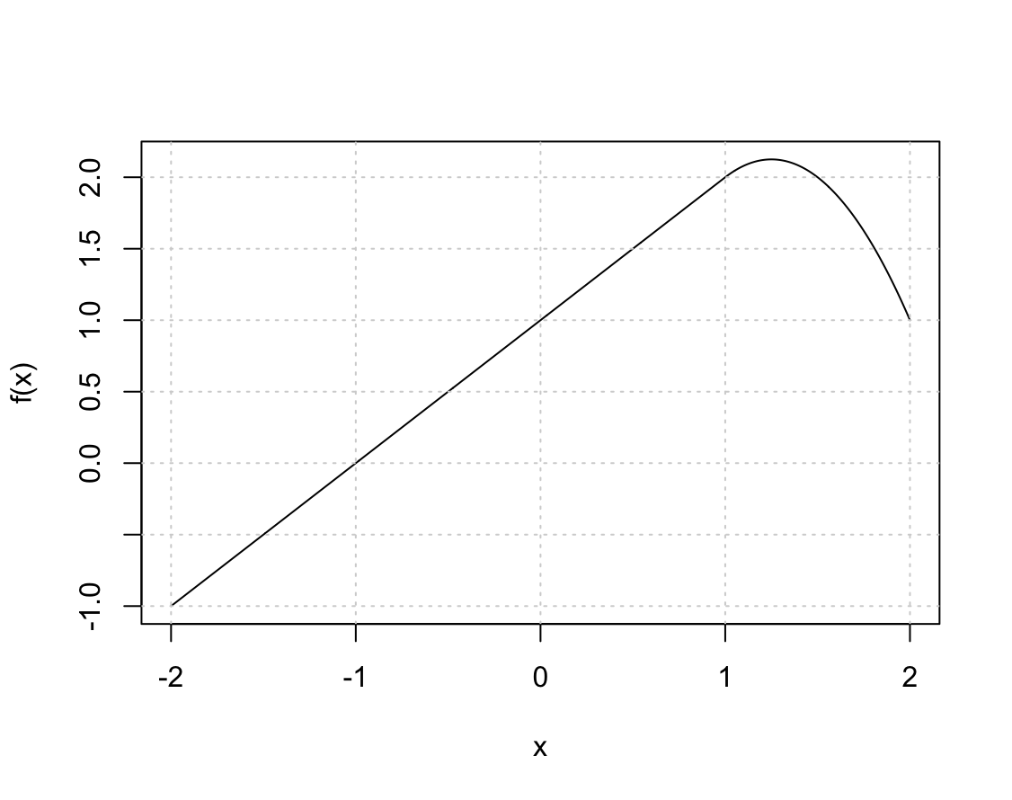
-
Suppose we fit a curve with basis functions $b_1(X) = I(0 \le X \le 2) - (X-1)I(1 \le X \le 2)$, $b_2(X) = (X-3)I(3 \le X \le 4) + I(4 < X \le 5)$. We fit the linear regression model \(Y = \beta_0 + \beta_1 b_1(X) + \beta_2 b_2(X) + \epsilon,\)
and obtain coefficient estimates $\hat{\beta}_0 = 1$, $\hat{\beta}_1 = 1$, $\hat{\beta}_2 = 3$. Sketch the estimated curve between $X = -2$ and $X = 6$. Note the intercepts, slopes, and other relevant information.
 x <- seq(-2, 6, length.out = 1000)
 b1 <- function(x) I(0 <= x & x <= 2) - (x - 1) * I(1 <= x & x <= 2)
 b2 <- function(x) (x - 3) * I(3 <= x & x <= 4) + I(4 < x & x <= 5)
 f <- function(x) 1 + 1 * b1(x) + 3 * b2(x)
 plot(x, f(x), type = "l")
 grid()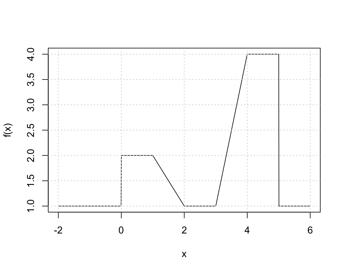
-
Consider two curves, $\hat{g}_1$ and $\hat{g}_2$, defined by
\[\hat{g}_1 = \arg\underset{g}{\min} \left( \sum_{i=1}^{n} (y_i - g(x_i))^2 + \lambda \int \left[g^{(3)}(x)\right]^2 dx \right),\] \[\hat{g}_2 = \arg\underset{g}{\min} \left( \sum_{i=1}^{n} (y_i - g(x_i))^2 + \lambda \int \left[g^{(4)}(x)\right]^2 dx \right),\]where $g^{(m)}$ represents the $m$th derivative of $g$.
(a) As $\lambda \to \infty$, will $\hat{g}_1$ or $\hat{g}_2$ have the smaller training RSS?
$\hat{g}_2$ jest bardziej elastyczne dlatego, że korzysta z pochodnej wyższego rzędu, dlatego będzie miało mniejsze RSS na zbiorze treningowym.
(b) As $\lambda \to \infty$, will $\hat{g}_1$ or $\hat{g}_2$ have the smaller test RSS?
Nie można tego stwierdzić bez zbioru testowego.
(c) For $\lambda = 0$, will $\hat{g}_1$ or $\hat{g}_2$ have the smaller training and test RSS?
RSS będzie taki sam dla obu funkcji, bo drugi człon wynosi 0.
-
In this exercise, you will further analyze the
Wagedata set considered throughout this chapter.(a) Perform polynomial regression to predict
wageusingage. Use cross-validation to select the optimal degree d for the polynomial. What degree was chosen, and how does this compare to the results of hypothesis testing using ANOVA? Make a plot of the resulting polynomial fit to the data.library(ISLR2) library(boot) attach(Wage) cv.error <- rep(0, 10) for (i in 1:10) { glm.fit <- glm(wage ~ poly(age, i), data = Wage) cv.error[i] <- cv.glm(Wage, glm.fit, K = 10)$delta[1] } cv.error[1] 1676.826 1600.763 1598.399 1595.651 1594.977 1596.061 1594.298 [8] 1598.134 1593.913 1595.950plot(cv.error, type="b", xlab="Degree", ylab="CV Error")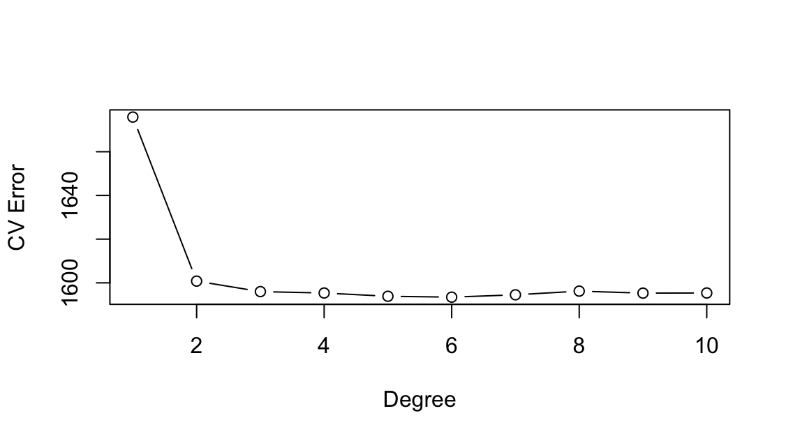
Nie widać poprawy modelu powyżej wielomianu 4 stopnia.
glm.fit = glm(wage ~ poly(age, 5), data = Wage) summary(glm.fit)Call: glm(formula = wage ~ poly(age, 5), data = Wage) Coefficients: Estimate Std. Error t value Pr(>|t|) (Intercept) 111.7036 0.7288 153.278 < 2e-16 *** poly(age, 5)1 447.0679 39.9161 11.200 < 2e-16 *** poly(age, 5)2 -478.3158 39.9161 -11.983 < 2e-16 *** poly(age, 5)3 125.5217 39.9161 3.145 0.00168 ** poly(age, 5)4 -77.9112 39.9161 -1.952 0.05105 . poly(age, 5)5 -35.8129 39.9161 -0.897 0.36968 --- Signif. codes: 0 ‘***’ 0.001 ‘**’ 0.01 ‘*’ 0.05 ‘.’ 0.1 ‘ ’ 1 (Dispersion parameter for gaussian family taken to be 1593.294) Null deviance: 5222086 on 2999 degrees of freedom Residual deviance: 4770322 on 2994 degrees of freedom AIC: 30642 Number of Fisher Scoring iterations: 2Na podstawie $p$-value 5 stopień wielomianu nie jest istotny statystycznie.
 fit1 <- lm(wage ~ poly(age, 1), data = Wage)
 fit2 <- lm(wage ~ poly(age, 2), data = Wage)
 fit3 <- lm(wage ~ poly(age, 3), data = Wage)
 fit4 <- lm(wage ~ poly(age, 4), data = Wage)
 fit5 <- lm(wage ~ poly(age, 5), data = Wage)
 anova(fit1, fit2, fit3, fit4, fit5)
Analysis of Variance Table Model 1: wage ~ poly(age, 1) Model 2: wage ~ poly(age, 2) Model 3: wage ~ poly(age, 3) Model 4: wage ~ poly(age, 4) Model 5: wage ~ poly(age, 5) Res.Df RSS Df Sum of Sq F Pr(>F) 1 2998 5022216 2 2997 4793430 1 228786 143.5931 < 2.2e-16 *** 3 2996 4777674 1 15756 9.8888 0.001679 ** 4 2995 4771604 1 6070 3.8098 0.051046 . 5 2994 4770322 1 1283 0.8050 0.369682 --- Signif. codes: 0 ‘***’ 0.001 ‘**’ 0.01 ‘*’ 0.05 ‘.’ 0.1 ‘ ’ 1Na podstawie $p$-value można stwierdzić, że model z wielomianem 5 stopnia nie jest istotny statystycznie. Ostatecznie trzeba wybrać model z wielomianem 4 stopnia.
 agelims <- range(age)
 age.grid <- seq(from = agelims[1], to = agelims[2])
 preds <- predict(fit4, newdata = list(age = age.grid ), se = TRUE )
 se.bands <- cbind(preds$fit + 2 * preds$se.fit,
                   preds$fit - 2 * preds$se.fit)

 plot(age, wage, xlim = agelims, cex = .5, col = "darkgrey")
 title("Degree -4 Polynomial")
 lines(age.grid, preds$fit, lwd = 2, col = "blue")
 matlines(age.grid, se.bands, lwd = 1, col = "blue", lty = 3)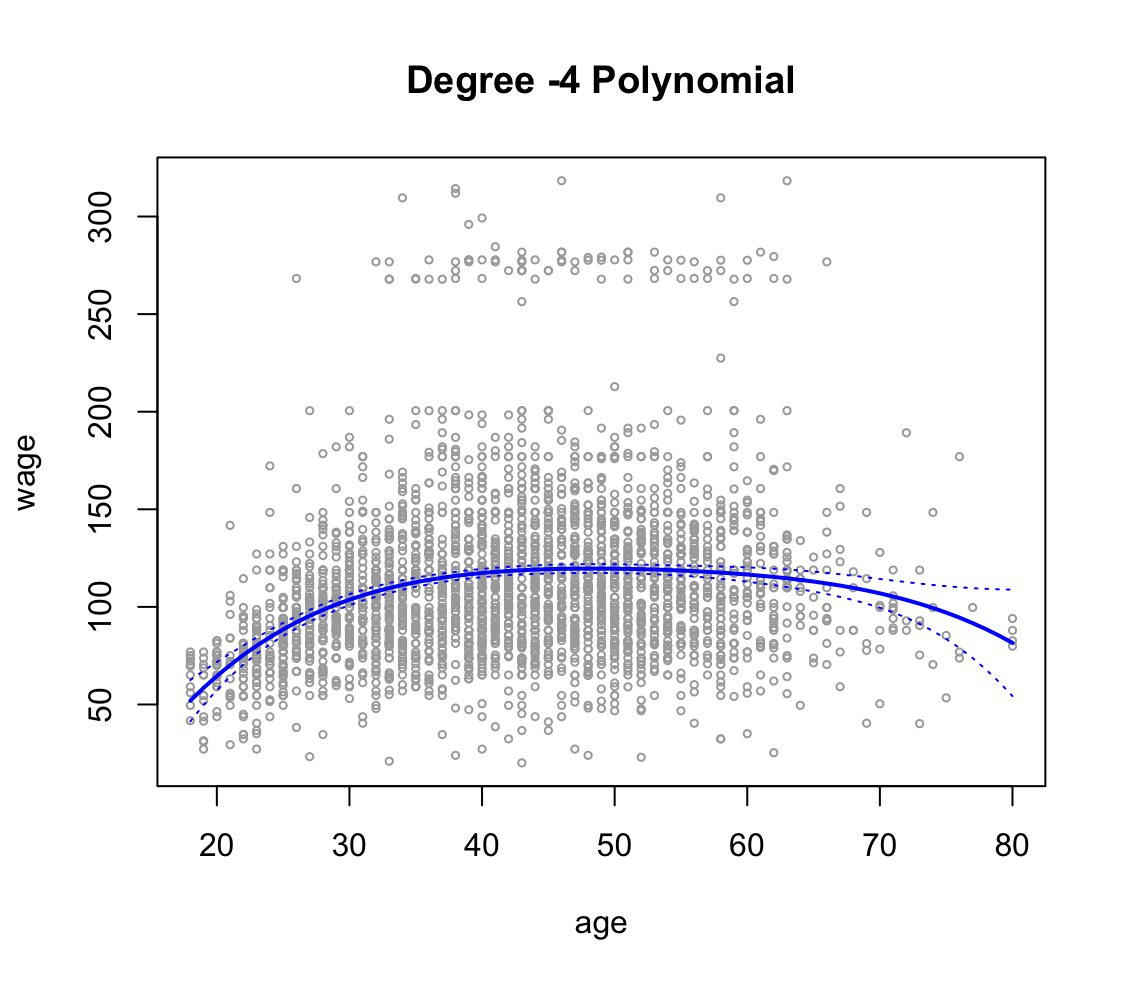
(b) Fit a step function to predict
wageusingage, and perform cross-validation to choose the optimal number of cuts. Make a plot of the fit obtained.Wage_2 <- Wage attach(Wage_2) set.seed(1) cv.error = rep(0,9) for (i in 2:10) { Wage_2$age.cut = cut(age, i) step.fit = glm(wage ~ age.cut, data = Wage_2) cv.error[i-1] = cv.glm(Wage_2, step.fit, K=10)$delta[1] } cv.error[1] 1734.489 1684.271 1635.552 1632.080 1623.415 1614.996 1601.318 [8] 1613.954 1606.331plot(2:10, cv.error, type="b", xlab="Index", ylab="CV Error")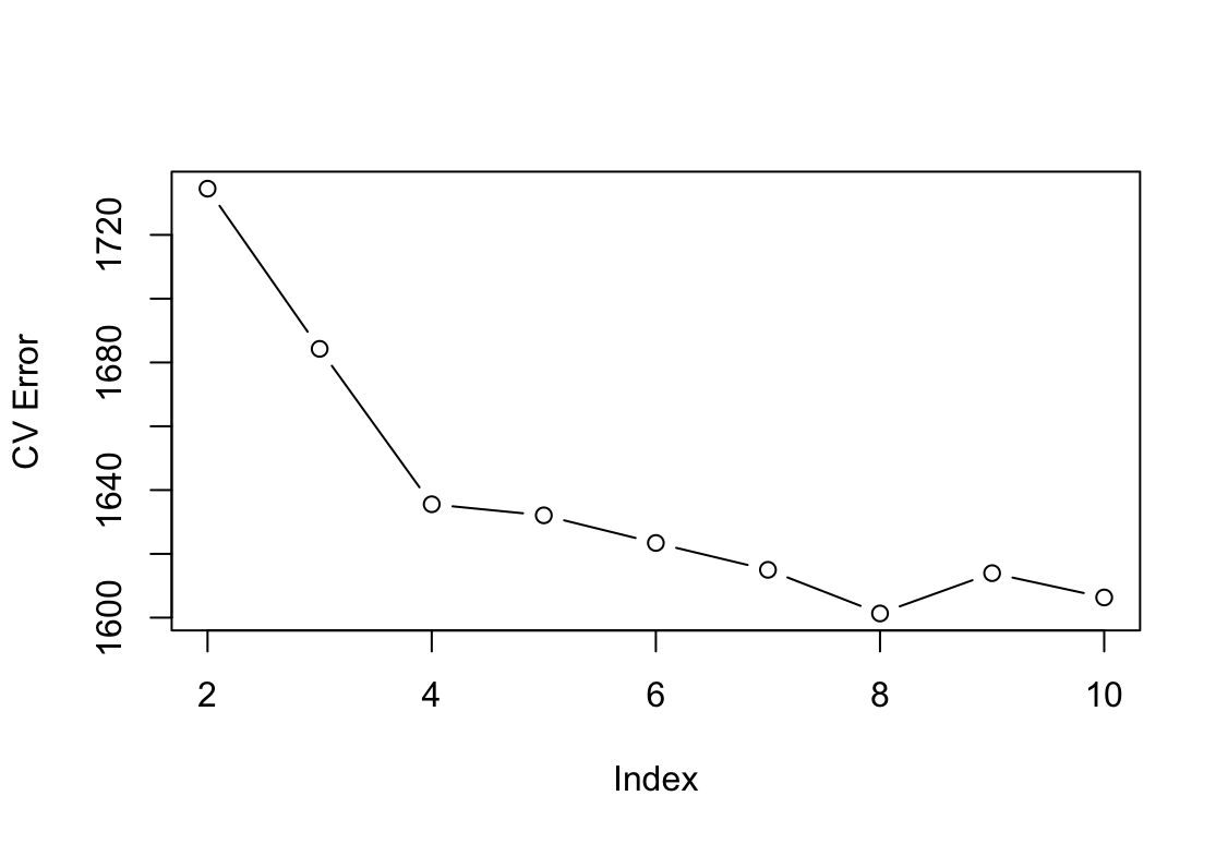
Najmniejszy błąd dla 8 podziałów.
 attach(Wage)
 step.fit <- glm(wage ~ cut(age, 8), data = Wage)

 preds <- predict(step.fit, newdata = list(age = age.grid), se = TRUE)
 se.bands <- cbind(preds$fit + 2 * preds$se.fit,
                   preds$fit - 2 * preds$se.fit)

 plot(age, wage, xlim = agelims, cex = .5, col = "darkgrey")
 title("Step function using 8 cuts")
 lines(age.grid, preds$fit, lwd = 2, col = "blue")
 matlines(age.grid, se.bands, lwd = 1, col = "blue", lty = 3)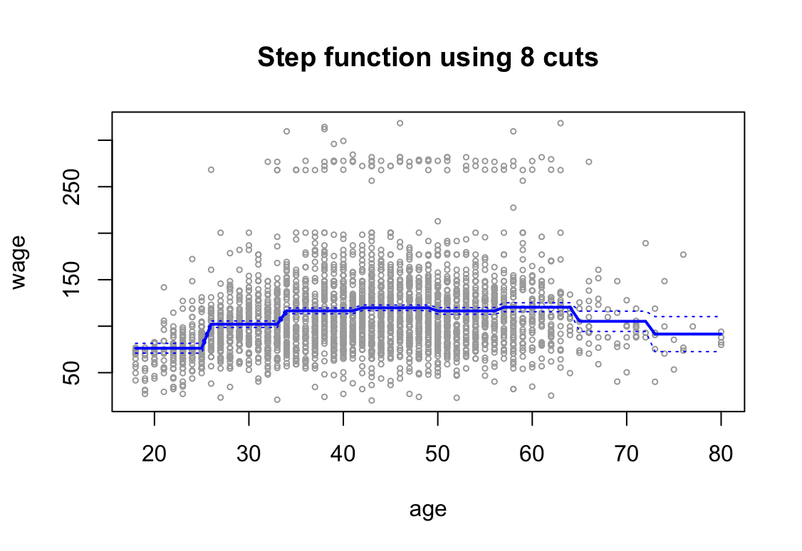
-
The
Wagedata set contains a number of other features not explored in this chapter, such as marital status (maritl), job class (jobclass), and others. Explore the relationships between some of these other predictors andwage, and use non-linear fitting techniques in order to fit flexible models to the data. Create plots of the results obtained, and write a summary of your findings.library(ISLR2) attach(Wage) plot(year, wage)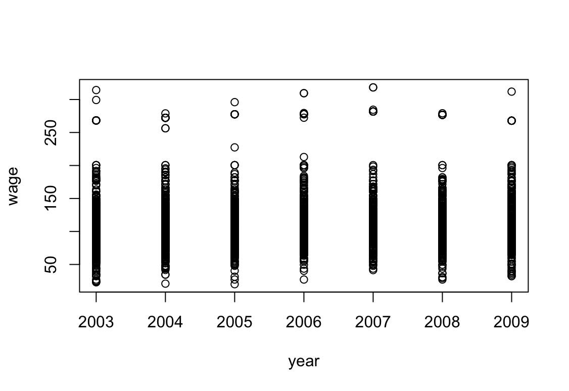
plot(age, wage)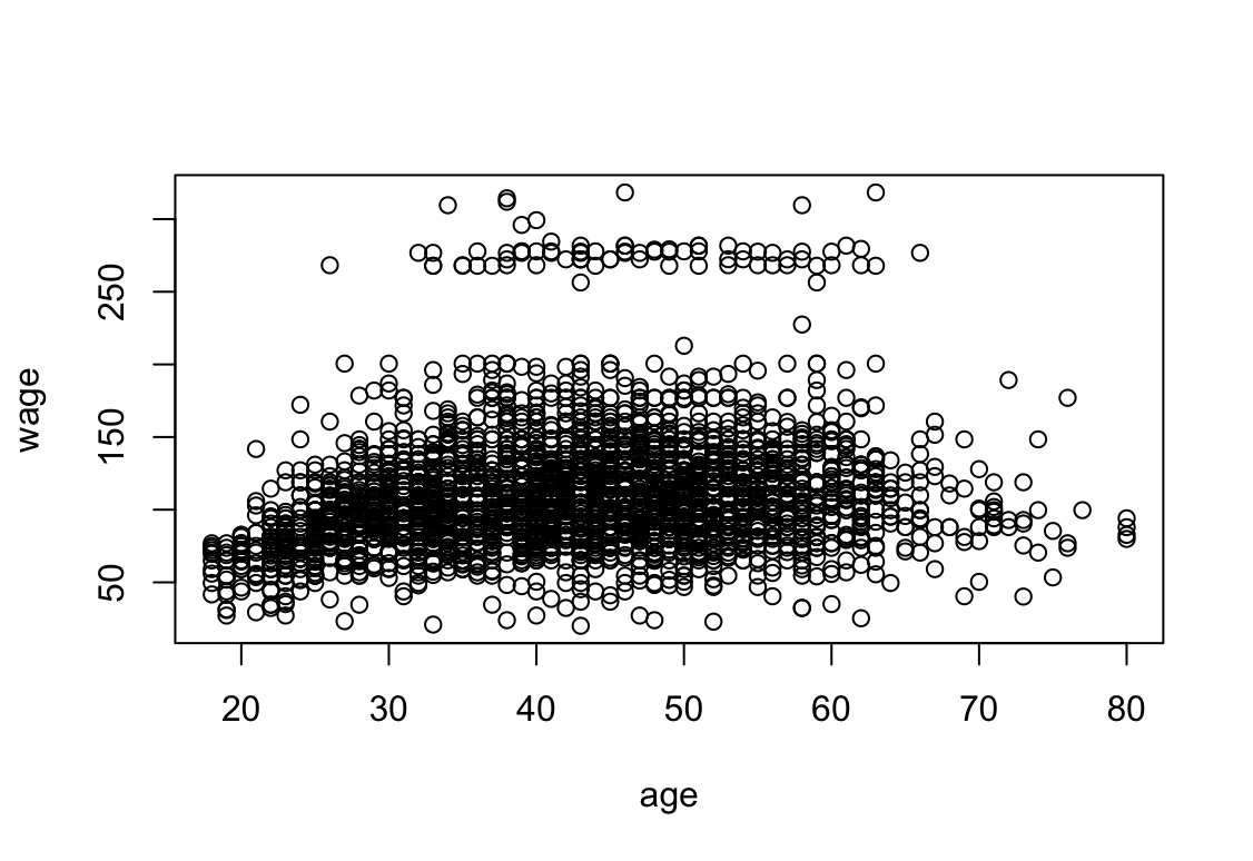
plot(maritl, wage)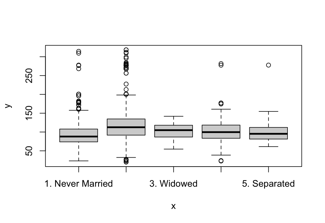
plot(jobclass, wage)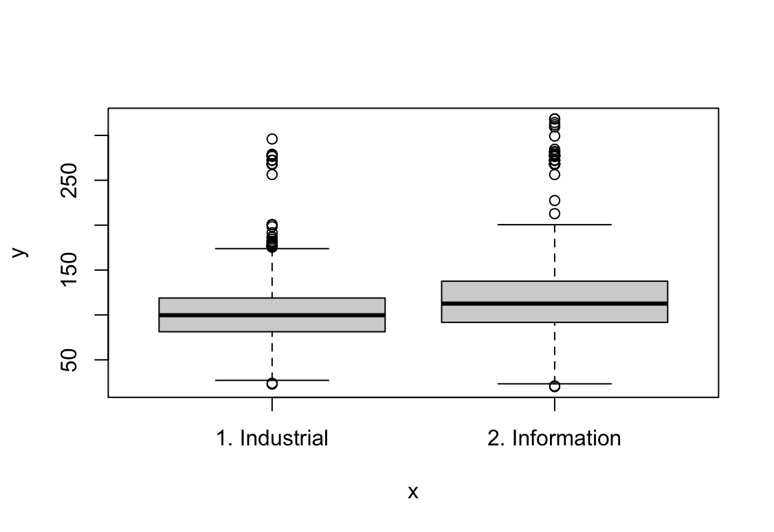
plot(education, wage)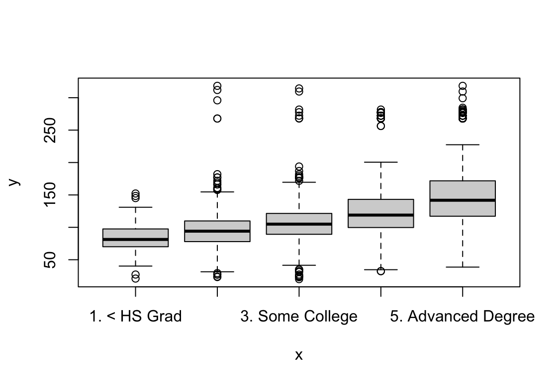
Jak widać zbiór danych
Wagezawiera zmienne ilościowe i jakościowe. Ponadto zmienne ilościowe nie są liniowe, więc dobrym wyborem do modelowania są modele GAM.library(gam) fit0 <- gam(wage ~ s(year, 4) + s(age, 5) + education, data = Wage) fit2 <- gam(wage ~ s(year, 4) + s(age, 5) + education + maritl, data = Wage) fit1 <- gam(wage ~ s(year, 4) + s(age, 5) + education + jobclass, data = Wage) fit3 <- gam(wage ~ s(year, 4) + s(age, 5) + education + jobclass + maritl, data = Wage) anova(fit0, fit1, fit2, fit3)Analysis of Deviance Table Model 1: wage ~ s(year, 4) + s(age, 5) + education Model 2: wage ~ s(year, 4) + s(age, 5) + education + jobclass Model 3: wage ~ s(year, 4) + s(age, 5) + education + maritl Model 4: wage ~ s(year, 4) + s(age, 5) + education + jobclass + maritl Resid. Df Resid. Dev Df Deviance Pr(>Chi) 1 2986 3689770 2 2985 3677553 1 12218 0.0014286 ** 3 2982 3595688 3 81865 1.071e-14 *** 4 2981 3581781 1 13907 0.0006687 *** --- Signif. codes: 0 ‘***’ 0.001 ‘**’ 0.01 ‘*’ 0.05 ‘.’ 0.1 ‘ ’ 1Model z największą liczbą zmiennych nadal jest istotny statystycznie.
 par(mfrow = c(2, 3))
 plot(fit3, se = TRUE, col = "blue")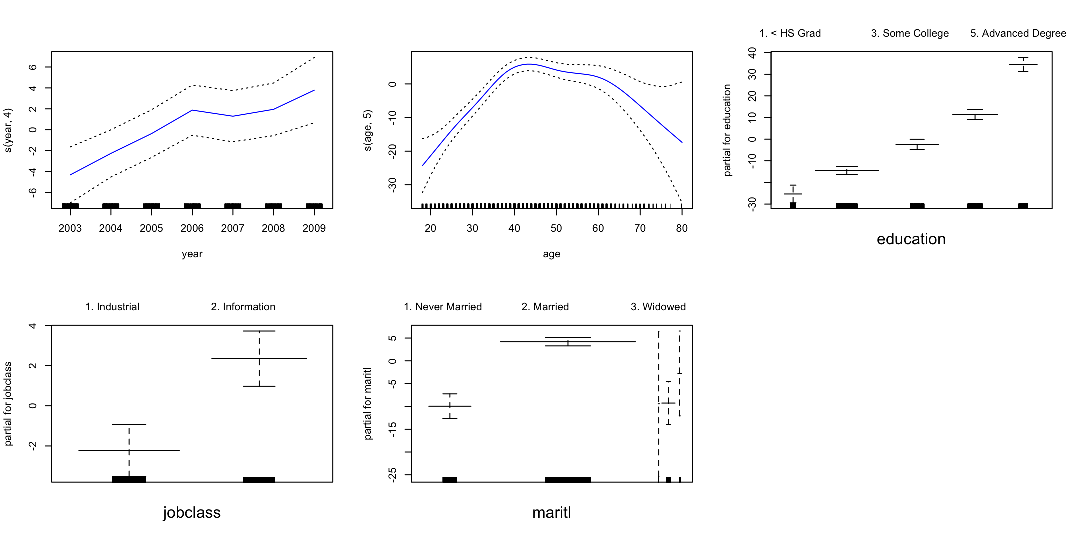
Wynik pokazuje, że pensja rośnie wraz z każdym kolejnym rokiem kiedy weźmiemy ustalone wartości pozostałych zmiennych. W przypadku wieku pensja jest najwyższa dla ludzi w wieku ok. 42 lat. Wyższa edukacja pozwala na uzyskanie wyższych zarobków. Praca w usługach jest lepiej płatna. Zarobki osób po ślubie są wyższe, dla wdowców i osób w separacji widzimy szeroki zakres błędu standardowego.
-
Fit some of the non-linear models investigated in this chapter to the
Autodata set. Is there evidence for non-linear relationships in this data set? Create some informative plots to justify your answer.library(ISLR2) attach(Auto) pairs(Auto[1:7])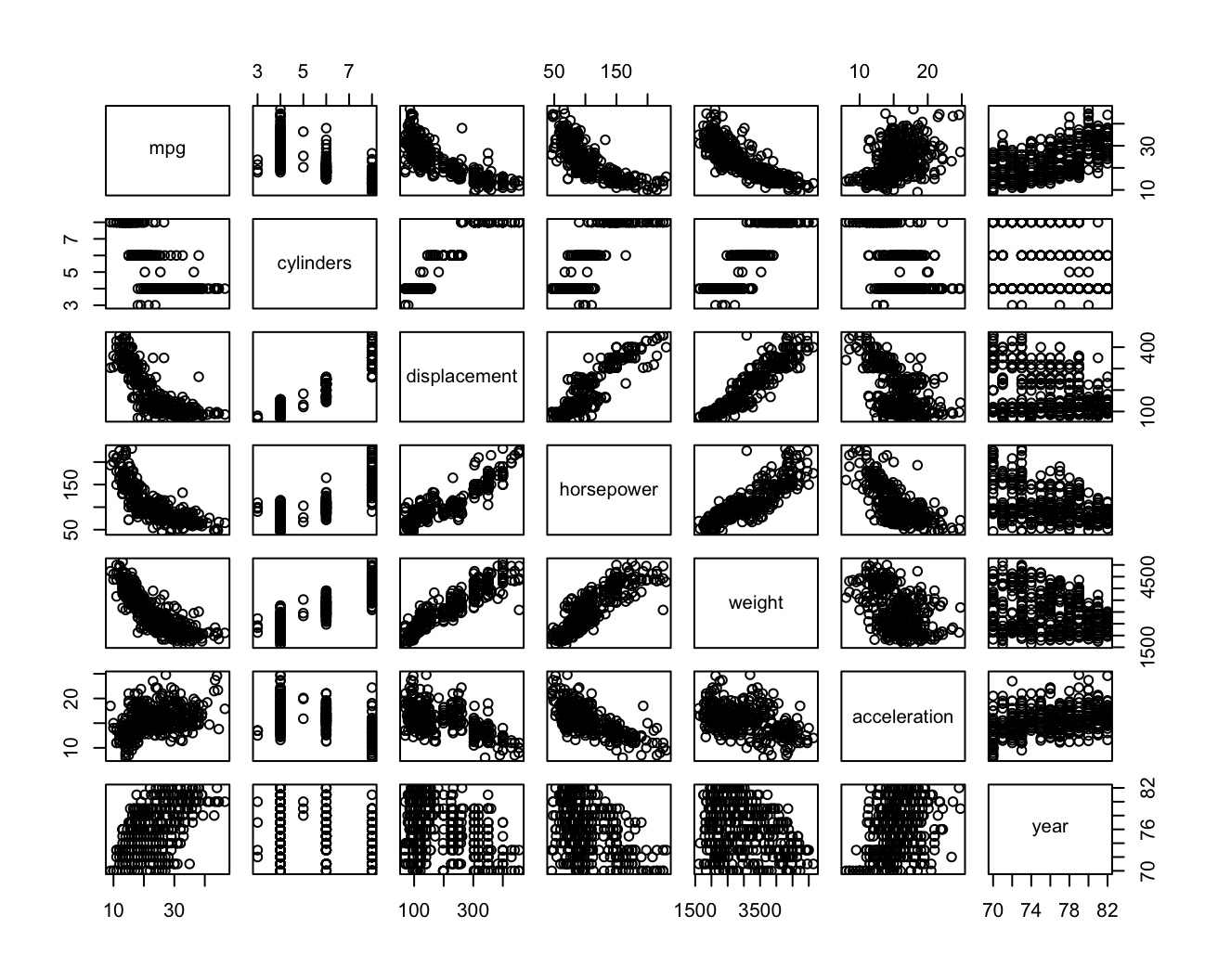
Widać nieliniową zależność między zmiennymi
mpg,displacement/horsepower/weight. Dopasuję model wielomianowy do zmiennychmpgihorsepower.fit.1 = lm(mpg ~ poly(horsepower, 1), data = Auto) fit.2 = lm(mpg ~ poly(horsepower, 2), data = Auto) fit.3 = lm(mpg ~ poly(horsepower, 3), data = Auto) fit.4 = lm(mpg ~ poly(horsepower, 4), data = Auto) fit.5 = lm(mpg ~ poly(horsepower, 5), data = Auto) fit.6 = lm(mpg ~ poly(horsepower, 6), data = Auto) anova(fit.1, fit.2, fit.3, fit.4, fit.5, fit.6)Analysis of Variance Table Model 1: mpg ~ poly(horsepower, 1) Model 2: mpg ~ poly(horsepower, 2) Model 3: mpg ~ poly(horsepower, 3) Model 4: mpg ~ poly(horsepower, 4) Model 5: mpg ~ poly(horsepower, 5) Model 6: mpg ~ poly(horsepower, 6) Res.Df RSS Df Sum of Sq F Pr(>F) 1 390 9385.9 2 389 7442.0 1 1943.89 104.6659 < 2.2e-16 *** 3 388 7426.4 1 15.59 0.8396 0.360083 4 387 7399.5 1 26.91 1.4491 0.229410 5 386 7223.4 1 176.15 9.4846 0.002221 ** 6 385 7150.3 1 73.04 3.9326 0.048068 * --- Signif. codes: 0 ‘***’ 0.001 ‘**’ 0.01 ‘*’ 0.05 ‘.’ 0.1 ‘ ’ 1Z ANOVY wynika, że odpowiedni będzie model kwadratowy.
summary(fit.2)Call: lm(formula = mpg ~ poly(horsepower, 2), data = Auto) Residuals: Min 1Q Median 3Q Max -14.7135 -2.5943 -0.0859 2.2868 15.8961 Coefficients: Estimate Std. Error t value Pr(>|t|) (Intercept) 23.4459 0.2209 106.13 <2e-16 *** poly(horsepower, 2)1 -120.1377 4.3739 -27.47 <2e-16 *** poly(horsepower, 2)2 44.0895 4.3739 10.08 <2e-16 *** --- Signif. codes: 0 ‘***’ 0.001 ‘**’ 0.01 ‘*’ 0.05 ‘.’ 0.1 ‘ ’ 1 Residual standard error: 4.374 on 389 degrees of freedom Multiple R-squared: 0.6876, Adjusted R-squared: 0.686 F-statistic: 428 on 2 and 389 DF, p-value: < 2.2e-16 -
This question uses the variables
dis(the weighted mean of distances to five Boston employment centers) andnox(nitrogen oxides concentration in parts per 10 million) from theBostondata. We will treatdisas the predictor andnoxas the response.(a) Use the
poly()function to fit a cubic polynomial regression to predictnoxusingdis. Report the regression output, and plot the resulting data and polynomial fits.library(ISLR2) attach(Boston) fit <- glm(nox ~ poly(dis, 3), data = Boston) summary(fit)Call: glm(formula = nox ~ poly(dis, 3), data = Boston) Coefficients: Estimate Std. Error t value Pr(>|t|) (Intercept) 0.554695 0.002759 201.021 < 2e-16 *** poly(dis, 3)1 -2.003096 0.062071 -32.271 < 2e-16 *** poly(dis, 3)2 0.856330 0.062071 13.796 < 2e-16 *** poly(dis, 3)3 -0.318049 0.062071 -5.124 4.27e-07 *** --- Signif. codes: 0 ‘***’ 0.001 ‘**’ 0.01 ‘*’ 0.05 ‘.’ 0.1 ‘ ’ 1 (Dispersion parameter for gaussian family taken to be 0.003852802) Null deviance: 6.7810 on 505 degrees of freedom Residual deviance: 1.9341 on 502 degrees of freedom AIC: -1370.9 Number of Fisher Scoring iterations: 2lims <- range(dis) grid <- seq(from = lims[1], to = lims[2], 0.1) preds <- predict(fit, newdata = list(dis = grid), se = TRUE) se.bands <- cbind(preds$fit + 2 * preds$se.fit, preds$fit - 2 * preds$se.fit) plot(dis, nox, xlim = lims, cex = .5, col = "darkgrey") title("Degree -3 Polynomial") lines(grid, preds$fit, lwd = 2, col = "blue") matlines(grid, se.bands, lwd = 1, col = "blue", lty = 3)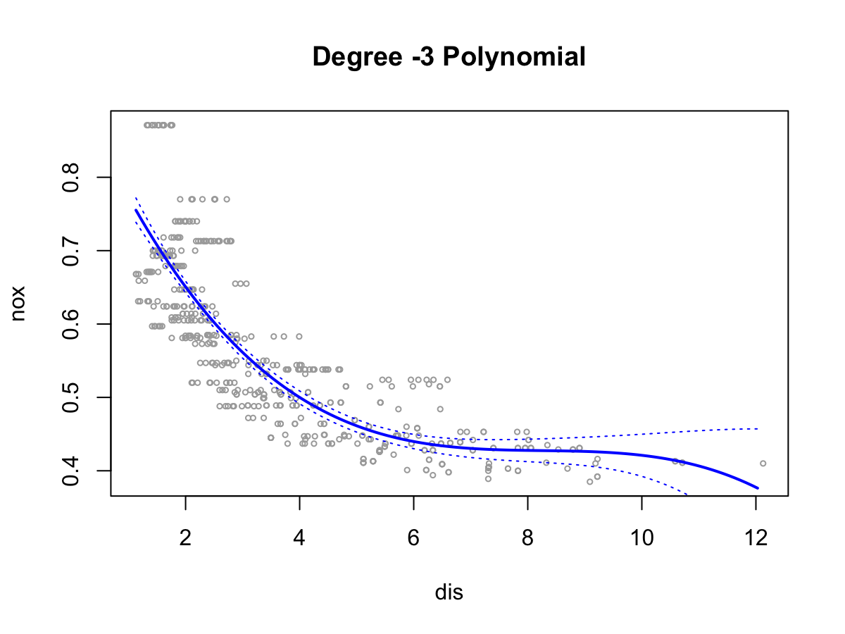
(b) Plot the polynomial fits for a range of different polynomial degrees (say, from 1 to 10), and report the associated residual sum of squares.
plot(dis, nox, xlim = lims, cex = .5, col = "darkgrey") title("Polynomial fits from degree 1-10.") colours = rainbow(10) rss = rep(0,10) set.seed(1) for (i in 1:10){ fit <- glm(nox ~ poly(dis, i), data = Boston) preds <- predict(fit, newdata = list(dis = grid), se = TRUE) lines(grid, preds$fit, lwd = 1.5, col = colours[i]) rss[i] = sum((nox - predict(fit, newdata = list(dis = dis)))^2) } legend(x=10, y=0.85,legend=1:10, col= colours[1:10],lwd=2) rss[1] 2.768563 2.035262 1.934107 1.932981 1.915290 1.878257 1.849484 1.835630 [9] 1.833331 1.832171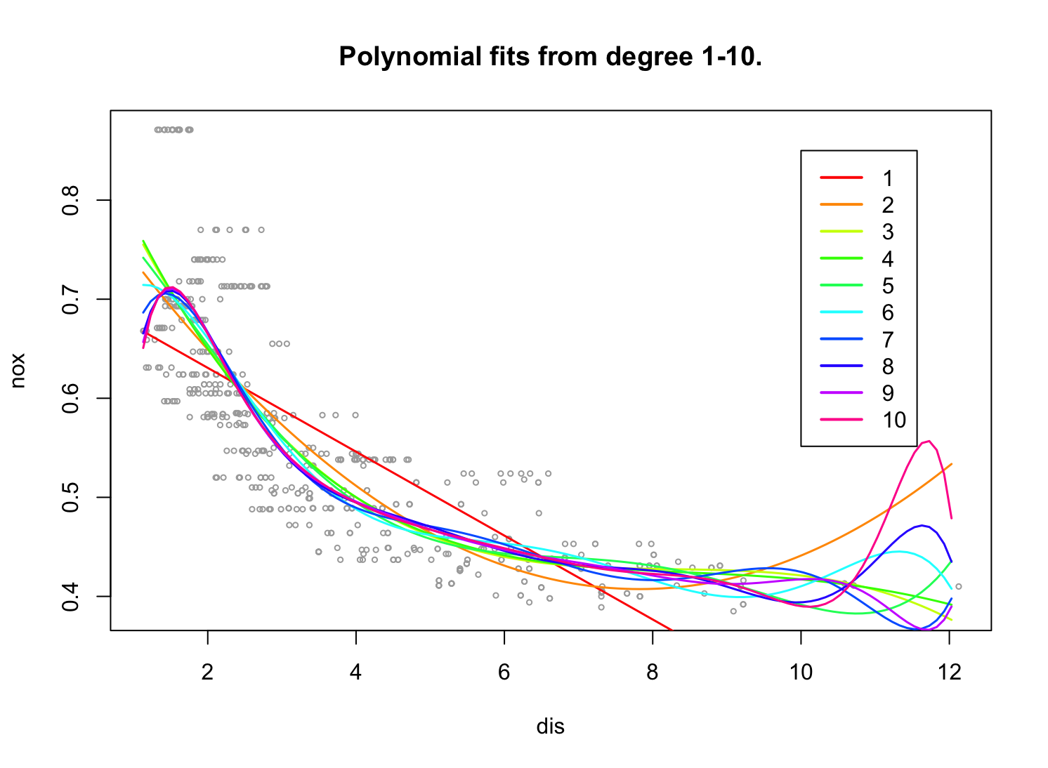
(c) Perform cross-validation or another approach to select the optimal degree for the polynomial, and explain your results.
library(boot) set.seed(1) cv.error <- rep(0, 10) for (i in 1:10) { fit <- glm(nox ~ poly(dis, i), data = Boston) cv.error[i] <- cv.glm(Boston, fit, K = 10)$delta[1] } which.min(cv.error)[1] 4(d) Use the
bs()function to fit a regression spline to predictnoxusingdis. Report the output for the fit using four degrees of freedom. How did you choose the knots? Plot the resulting fit.library(splines) fit <- glm(nox ~ bs(dis, df = 4), data = Boston) summary(fit)Call: glm(formula = nox ~ bs(dis, df = 4), data = Boston) Coefficients: Estimate Std. Error t value Pr(>|t|) (Intercept) 0.73447 0.01460 50.306 < 2e-16 *** bs(dis, df = 4)1 -0.05810 0.02186 -2.658 0.00812 ** bs(dis, df = 4)2 -0.46356 0.02366 -19.596 < 2e-16 *** bs(dis, df = 4)3 -0.19979 0.04311 -4.634 4.58e-06 *** bs(dis, df = 4)4 -0.38881 0.04551 -8.544 < 2e-16 *** --- Signif. codes: 0 ‘***’ 0.001 ‘**’ 0.01 ‘*’ 0.05 ‘.’ 0.1 ‘ ’ 1 (Dispersion parameter for gaussian family taken to be 0.003837874) Null deviance: 6.7810 on 505 degrees of freedom Residual deviance: 1.9228 on 501 degrees of freedom AIC: -1371.9 Number of Fisher Scoring iterations: 2Wszystkie stopnie swobody są istotne statystycznie na podstawie $p$-value.
attr(bs(Boston$dis, df = 4), "knots")[1] 3.20745Węzły wybierane są automatycznie na podstawie kwantyli.
 preds <- predict(fit, newdata = list(dis = grid), se = TRUE)
 se.bands <- cbind(preds$fit + 2 * preds$se.fit,
                   preds$fit - 2 * preds$se.fit)

 plot(dis, nox, xlim = lims, cex = .5, col = "darkgrey")
 title("Regression spline")
 lines(grid, preds$fit, lwd = 2, col = "blue")
 matlines(grid, se.bands, lwd = 1, col = "blue", lty = 3)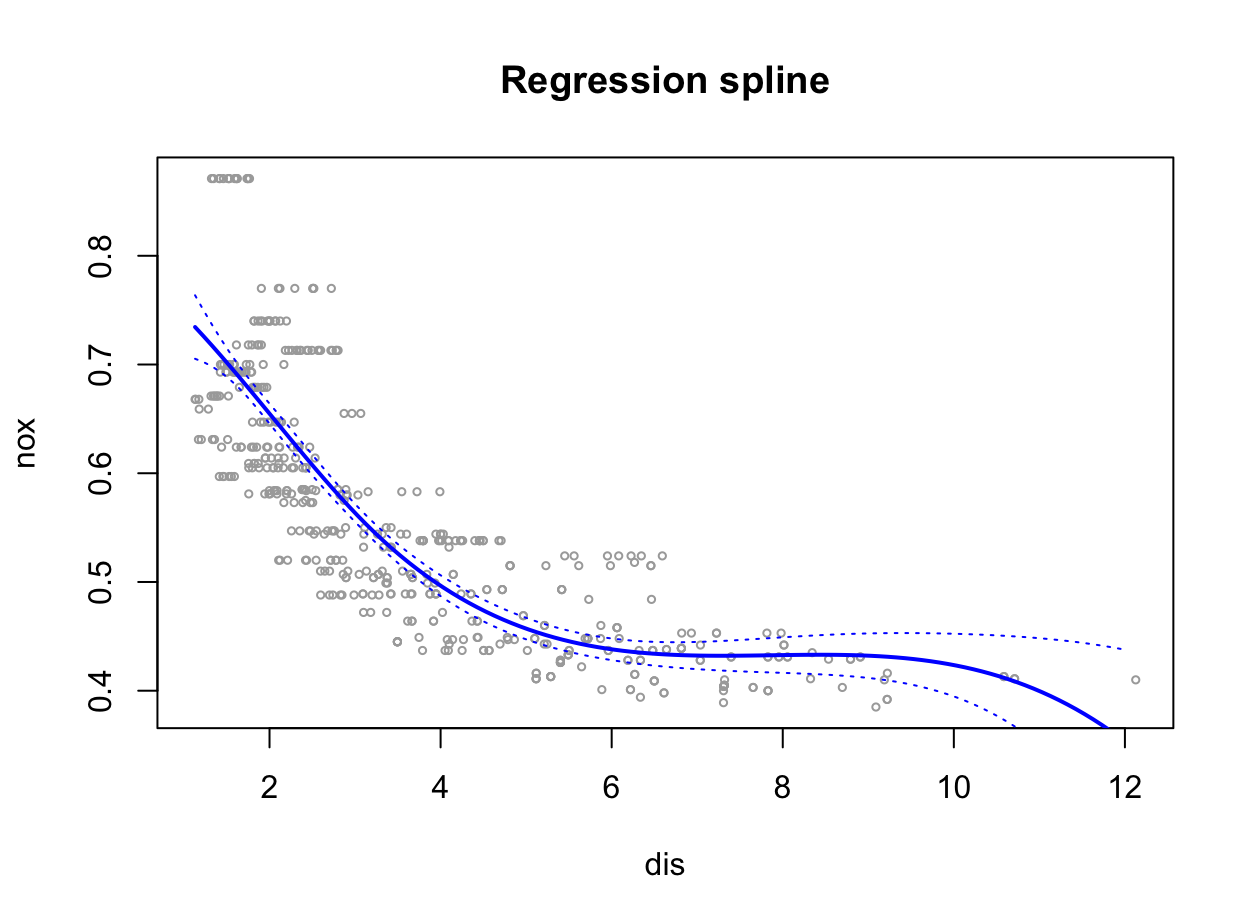
(e) Now fit a regression spline for a range of degrees of freedom, and plot the resulting fits and report the resulting RSS. Describe the results obtained.
plot(dis, nox, xlim = lims, cex = .5, col = "darkgrey") title("Splines fits from degree 1-10.") colours = rainbow(10) rss = rep(0,10) set.seed(1) for (i in 1:10){ fit <- glm(nox ~ bs(dis, df = i), data = Boston) preds <- predict(fit, newdata = list(dis = grid), se = TRUE) lines(grid, preds$fit, lwd = 1.5, col = colours[i]) rss[i] <- sum((nox - predict(fit, newdata = list(dis = dis)))^2) } legend(x = 10, y = 0.85, legend = 1:10, col = colours[1:10], lwd = 2) rss[1] 1.934107 1.934107 1.934107 1.922775 1.840173 1.833966 1.829884 1.816995 [9] 1.825653 1.792535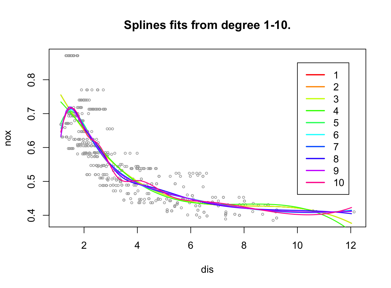
RSS są niższe niż w przypadku modeli wielomianowych. Widać, że modele z większą liczbą stopni swobody są przetrenowane.
(f) Perform cross-validation or another approach in order to select the best degrees of freedom for a regression spline on this data. Describe your results.
set.seed(1) cv.error <- rep(0, 10) for (i in 1:10) { fit <- glm(nox ~ bs(dis, df = i), data = Boston) cv.error[i] <- cv.glm(Boston, fit, K = 10)$delta[1] } which.min(cv.error)[1] 10 -
This question relates to the
Collegedata set.(a) Split the data into a training set and a test set. Using out-of-state tuition as the response and the other variables as the predictors, perform forward stepwise selection on the training set in order to identify a satisfactory model that uses just a subset of the predictors.
library(ISLR2) library(leaps) attach(College) train <- sample(nrow(College), nrow(College) * 4 / 5) fit.fwd <- regsubsets(Outstate~., data = College[train, ], nvmax=17, method="forward") plot(summary(fit.fwd)$bic, type = "b") which.min(summary(fit.fwd)$bic)[1] 12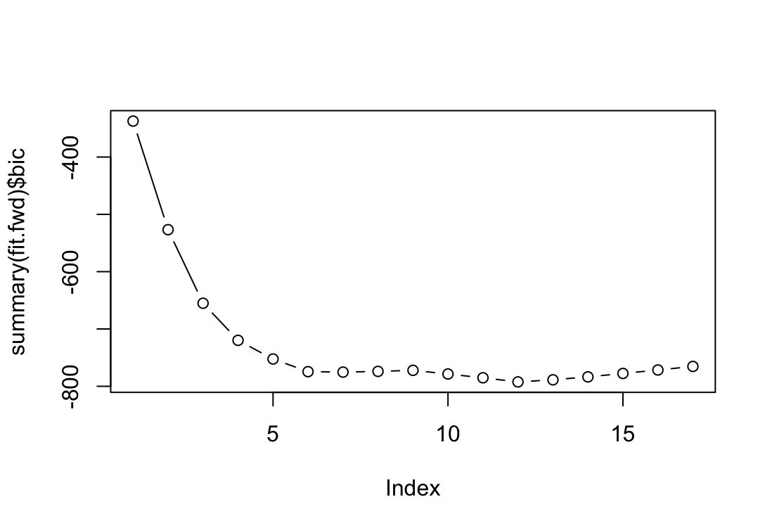
Najlepszy jest model zawierający 12 zmiennych ale powyżejsz 6 nie ma już znaczącej poprawy. Dla ułatwienia wybieram model z 6 zmiennymi.
coef(fit.fwd, id = 6)(Intercept) PrivateYes Room.Board PhD perc.alumni -3423.9571808 2793.7915223 0.9366486 35.4629229 45.2581015 Expend Grad.Rate 0.2148418 32.1605523(b) Fit a GAM on the training data, using out-of-state tuition as the response and the features selected in the previous step as the predictors. Plot the results, and explain your findings.
library(gam)
fit <- gam(Outstate ~ Private + s(Room.Board, 4) + s(PhD, 4) +
           s(perc.alumni, 2) + s(Expend, 4) + s(Grad.Rate, 5),
           data=College[train, ])

par(mfrow = c(2, 3))
plot(fit, col = "blue", se = TRUE)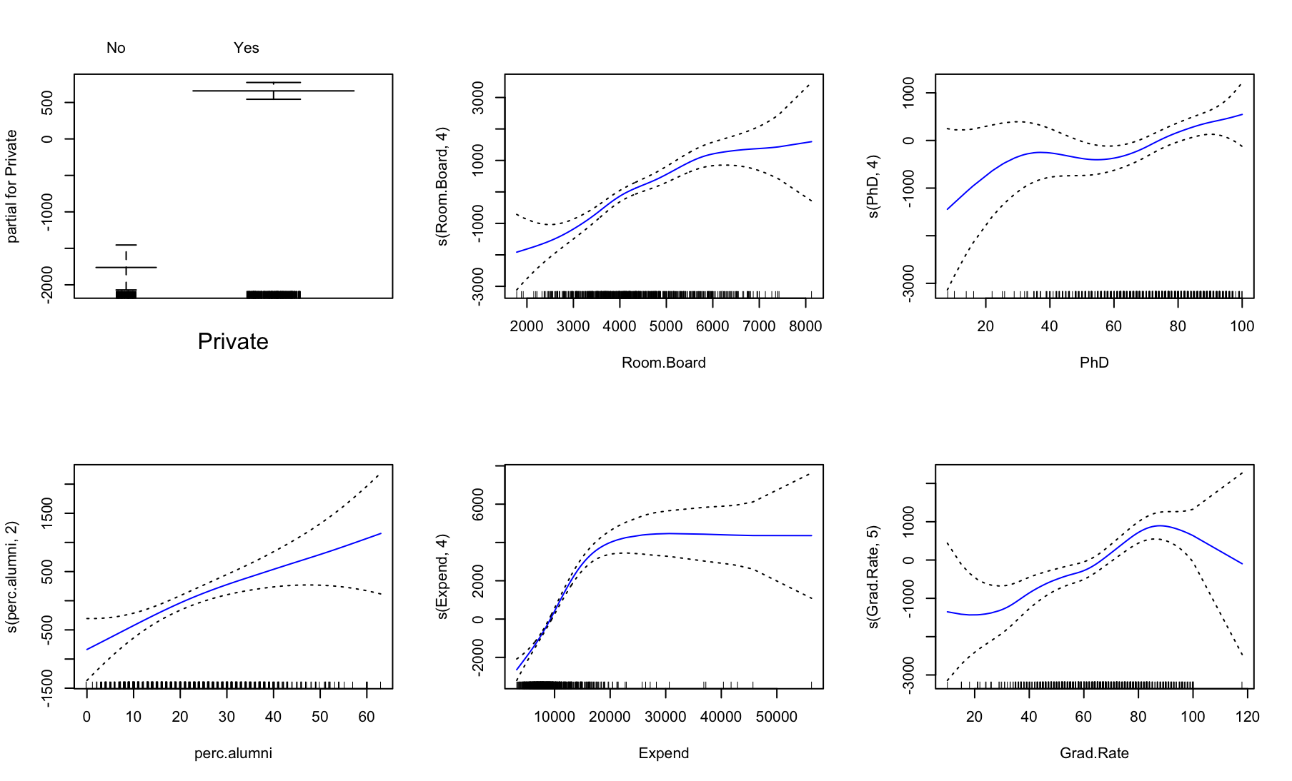
(c) Evaluate the model obtained on the test set, and explain the results obtained.
preds = predict(fit, newdata = College[-train, ]) # r-squared 1 - mean((College[-train, ]$Outstate - preds)^2) / mean((College[-train, ]$Outstate - mean(College[-train, ]$Outstate))^2)[1] 0.8057576Na podstawie $R^2$ model jest dobry.
(d) For which variables, if any, is there evidence of a non-linear relationship with the response?
summary(fit)Call: gam(formula = Outstate ~ Private + s(Room.Board, 4) + s(PhD, 4) + s(perc.alumni, 2) + s(Expend, 4) + s(Grad.Rate, 5), data = College[train, ]) Deviance Residuals: Min 1Q Median 3Q Max -7319.03 -1141.45 21.32 1274.46 7642.76 (Dispersion Parameter for gaussian family taken to be 3484410) Null Deviance: 9851839741 on 620 degrees of freedom Residual Deviance: 2090645450 on 599.9998 degrees of freedom AIC: 11139.58 Number of Local Scoring Iterations: NA Anova for Parametric Effects Df Sum Sq Mean Sq F value Pr(>F) Private 1 2490518062 2490518062 714.760 < 2.2e-16 *** s(Room.Board, 4) 1 1838285948 1838285948 527.574 < 2.2e-16 *** s(PhD, 4) 1 591148840 591148840 169.655 < 2.2e-16 *** s(perc.alumni, 2) 1 386891415 386891415 111.035 < 2.2e-16 *** s(Expend, 4) 1 855784793 855784793 245.604 < 2.2e-16 *** s(Grad.Rate, 5) 1 135641164 135641164 38.928 8.31e-10 *** Residuals 600 2090645450 3484410 --- Signif. codes: 0 ‘***’ 0.001 ‘**’ 0.01 ‘*’ 0.05 ‘.’ 0.1 ‘ ’ 1 Anova for Nonparametric Effects Npar Df Npar F Pr(F) (Intercept) Private s(Room.Board, 4) 3 2.824 0.03806 * s(PhD, 4) 3 1.900 0.12837 s(perc.alumni, 2) 1 0.831 0.36223 s(Expend, 4) 3 39.302 < 2e-16 *** s(Grad.Rate, 5) 4 2.130 0.07568 . --- Signif. codes: 0 ‘***’ 0.001 ‘**’ 0.01 ‘*’ 0.05 ‘.’ 0.1 ‘ ’ 1Nieliniowość jest istotna statystycznie dla zmiennych
Room.BoardiExpend. -
In Section 7.7, it was mentioned that GAMs are generally fit using a backfitting approach. The idea behind backfitting is actually quite simple. We will now explore backfitting in the context of multiple linear regression.
Suppose that we would like to perform multiple linear regression, but we do not have software to do so. Instead, we only have software to perform simple linear regression. Therefore, we take the following iterative approach: we repeatedly hold all but one coefficient estimate fixed at its current value, and update only that coefficient estimate using a simple linear regression. The process is continued until convergence—that is, until the coefficient estimates stop changing.
We now try this out on a toy example.
(a) Generate a response $Y$ and two predictors $X_1$ and $X_2$, with $n = 100$.
set.seed(42)
x1 <- rnorm(100)
x2 <- rnorm(100)
y <- 2 + 0.2 * x1 + 4 * x2 + rnorm(100)
(b) Initialize $\hat{\beta}_1$ to take on a value of your choice. It does not matter what value you choose.
beta1 <- 20(c) Keeping $\hat{\beta}_1$ fixed, fit the model
\[\hat{Y} - \hat{\beta}_1 X_1 = \beta_0 + \beta_2 X_2 + \epsilon\]You can do this as follows:
> a <- y - beta1 * x1
> beta2 <- lm(a ~ x2)$coef[2]
a <- y - beta1 * x1 beta2 <- lm(a ~ x2)$coef[2](d) Keeping $\hat{\beta}_2$ fixed, fit the model
\[\hat{Y} - \hat{\beta}_2 X_2 = \beta_0 + \beta_1 X_1 + \epsilon\]You can do this as follows:
> a <- y - beta2 * x2
> beta1 <- lm(a∼ x1)$coef[2]
a <- y - beta2 * x2 beta1 <- lm(a ~ x1)$coef[2](e) Write a for loop to repeat (c) and (d) 1,000 times. Report the estimates of $\hat{\beta}_0$, $\hat{\beta}_1$, and $\hat{\beta}_2$ at each iteration of the for loop. Create a plot in which each of these values is displayed, with $\hat{\beta}_0$, $\hat{\beta}_1$, and $\hat{\beta}_2$ each shown in a different color.
beta.df = data.frame("beta0" = rep(0, 1000), "beta1" = rep(0, 1000),
                     "beta2" = rep(0, 1000))

beta1 <- 20
for (i in 1:1000){
  a = y - beta1 * x1
  model = lm(a ~ x2)
  beta2 = model$coef[2]
  beta.df$beta2[i]=  beta2

  a = y - beta2 * x2
  model = lm(a ~ x1)
  beta1 <- model$coef[2]
  beta.df$beta1[i] = beta1
  beta.df$beta0[i] = model$coef[1]
}

plot(1:1000, beta.df$beta2, ylim = range(-0.5:4.5), type = 'b', cex = 0.5,
     col = "blue", xlab = "Iteration", ylab = "Value", log = "x")
title("Coefficients found by iterating.")
lines(1:1000, beta.df$beta1, col = "red", type = 'b', cex = 0.5)
lines(1:1000, beta.df$beta0, col = "green", type = 'b', cex = 0.5)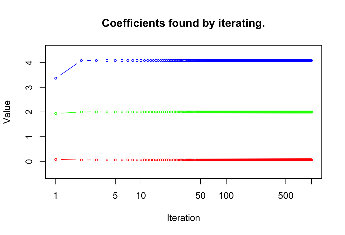
(f) Compare your answer in (e) to the results of simply performing multiple linear regression to predict $Y$ using $X_1$ and $X_2$. Use the
abline()function to overlay those multiple linear regression coefficient estimates on the plot obtained in (e).lm.fit = lm(y~ x1 + x2) coef(lm.fit)[1] plot(1:1000, beta.df$beta2, ylim = range(-0.5:4.5), type = 'b', cex = 0.5, col = "blue", xlab = "Iteration", ylab = "Value", log = "x") title("Coefficients found by standard method overlapped iteration.") lines(1:1000, beta.df$beta1, col = "red", type = 'b', cex = 0.5) lines(1:1000, beta.df$beta0, col = "green", type = 'b', cex = 0.5) abline(h = coef(lm.fit)[1]) abline(h = coef(lm.fit)[2]) abline(h = coef(lm.fit)[3])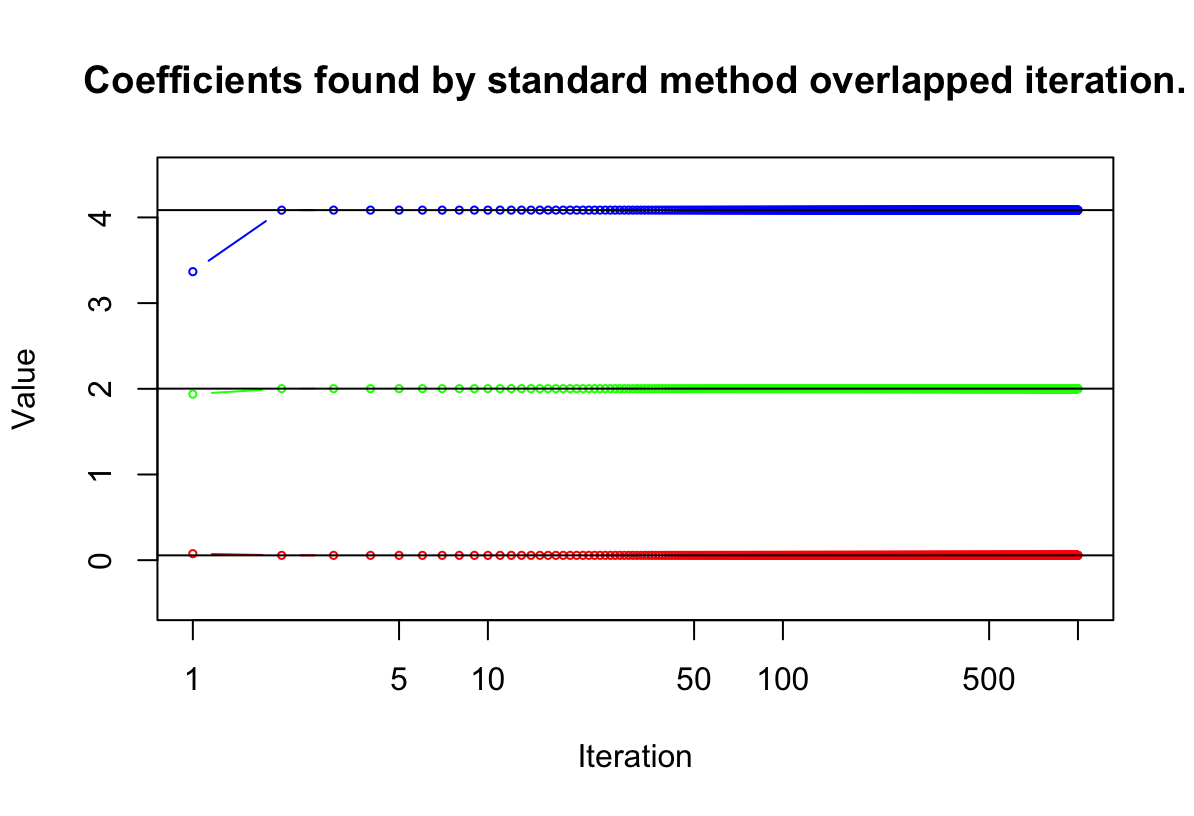
(g) On this data set, how many backfitting iterations were required in order to obtain a “good” approximation to the multiple regression coefficient estimates?
W tym przypadku potrzebne były 3 iteracje.
-
This problem is a continuation of the previous exercise. In a toy example with $p = 100$, show that one can approximate the multiple linear regression coefficient estimates by repeatedly performing simple linear regression in a backfitting procedure. How many backfitting iterations are required in order to obtain a “good” approximation to the multiple regression coefficient estimates? Create a plot to justify your answer.
set.seed(1)
p <- 100
n <- 1000

betas <- rnorm(p) * 5
x <- matrix(rnorm(n * p), ncol = p, nrow = n)
y <- 8 + (x %*% betas) + rnorm(n)

fit <- lm(y ~ x)

iter = 20
beta <- matrix(0, ncol = ncol(x), nrow = iter + 1)
for (i in 1:iter) {
  for (k in 1:ncol(x)) {
    residual <- y - (x[, -k] %*% beta[i, -k])
    beta[i + 1, k] <- lm(residual ~ x[, k])$coef[2]
  }
}

res <- beta[-1, ]
error <- rowMeans(sweep(res, 2, betas)^2)
plot(error, log = "x", type = "b")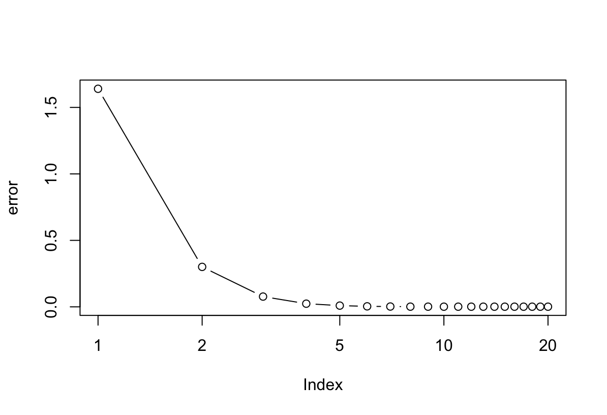
Potrzeba 6 iteracji żeby osiągnąć dobrą estymację parametrów.