Classification
-
Using a little bit of algebra, prove that (4.2) is equivalent to (4.3). In other words, the logistic function representation and logit representation for the logistic regression model are equivalent.
\[p(X)=\frac{e^{\beta_0+\beta_1 X}}{1+e^{\beta_0+\beta_1 X}}\] \[p(X) + p(X)e^{\beta_0+\beta_1 X}=e^{\beta_0+\beta_1 X}\] \[p(X) =e^{\beta_0+\beta_1 X} - p(X)e^{\beta_0+\beta_1 X}\] \[p(X) =e^{\beta_0+\beta_1 X}(1-p(X))\] \[\frac{p(X)}{1-p(X)} =e^{\beta_0+\beta_1 X}\] -
It was stated in the text that classifying an observation to the class for which (4.17) is largest is equivalent to classifying an observation to the class for which (4.18) is largest. Prove that this is the case. In other words, under the assumption that the observations in the kth class are drawn from a $N (\mu_k , \sigma^2)$ distribution, the Bayes classifier assigns an observation to the class for which the discriminant function is maximized.
\[p_k(x)=\frac{\pi_k \frac{1}{\sqrt{2 \pi} \sigma} \exp \left(-\frac{1}{2 \sigma^2}\left(x-\mu_k\right)^2\right)}{\sum_{l=1}^K \pi_l \frac{1}{\sqrt{2 \pi} \sigma} \exp \left(-\frac{1}{2 \sigma^2}\left(x-\mu_l\right)^2\right)}\] \[p_k(x)=\frac{\pi_k \frac{1}{\sqrt{2 \pi} \sigma} \exp \left(-\frac{1}{2 \sigma^2}\left(x^2-2x\mu_k + \mu_k^2\right)\right)}{\sum_{l=1}^K \pi_l \frac{1}{\sqrt{2 \pi} \sigma} \exp \left(-\frac{1}{2 \sigma^2}\left(x-\mu_l\right)^2\right)}\] \[p_k(x)=\frac{\frac{1}{\sqrt{2 \pi} \sigma} \exp \left(-\frac{x^2}{2 \sigma^2}\right)}{\sum_{l=1}^K \pi_l \frac{1}{\sqrt{2 \pi} \sigma} \exp \left(-\frac{1}{2 \sigma^2}\left(x-\mu_l\right)^2\right)} \cdot \pi_k \exp \left(\frac{x\mu_k}{\sigma^2}-\frac{\mu_k^2}{2\sigma^2}\right)\]Czynnik niezależny od $k$:
\[c=\frac{\frac{1}{\sqrt{2 \pi} \sigma} \exp \left(-\frac{x^2}{2 \sigma^2}\right)}{\sum_{l=1}^K \pi_l \frac{1}{\sqrt{2 \pi} \sigma} \exp \left(-\frac{1}{2 \sigma^2}\left(x-\mu_l\right)^2\right)}\] \[p_k(x)=c \pi_k \exp \left(\frac{x\mu_k}{\sigma^2}-\frac{\mu_k^2}{2\sigma^2}\right)\]Logarytmowanie:
\[\ln[p_k(x)]=\ln(c) + \ln(\pi_k) + \frac{x\mu_k}{\sigma^2} - \frac{\mu_k^2}{2\sigma^2}\]Ostatecznie:
\[\delta_k(x)=x\frac{\mu_k}{\sigma^2} - \frac{\mu_k^2}{2\sigma^2} + \ln(\pi_k)\] -
This problem relates to the QDA model, in which the observations within each class are drawn from a normal distribution with a class specific mean vector and a class specific covariance matrix. We consider the simple case where $p = 1$; i.e. there is only one feature.
Suppose that we have $K$ classes, and that if an observation belongs to the $k$th class then $X$ comes from a one-dimensional normal distribution, $X ∼ N(\mu_k, \sigma_k^2)$. Recall that the density function for the one-dimensional normal distribution is given in (4.16). Prove that in this case, the Bayes classifier is not linear. Argue that it is in fact quadratic.
Hint: For this problem, you should follow the arguments laid out in Section 4.4.1, but without making the assumption that $\sigma^2_1 =\ldots= \sigma_K^2$.
\[p_k(x)=\frac{\pi_k \frac{1}{\sqrt{2 \pi} \sigma_k} \exp \left(-\frac{1}{2 \sigma_k^2}\left(x^2-2x\mu_k + \mu_k^2\right)\right)}{\sum_{l=1}^K \pi_l \frac{1}{\sqrt{2 \pi} \sigma_l} \exp \left(-\frac{1}{2 \sigma_l^2}\left(x-\mu_l\right)^2\right)}\]Czynnik niezależny od $k$:
\[c=\frac{\frac{1}{\sqrt{2 \pi}}}{\sum_{l=1}^K \pi_l \frac{1}{\sqrt{2 \pi} \sigma_l} \exp \left(-\frac{1}{2 \sigma_l^2}\left(x-\mu_l\right)^2\right)}\] \[p_k(x)=c \frac{\pi_k}{\sigma_k} \exp \left(-\frac{1}{2 \sigma_k^2}\left(x^2-2x\mu_k + \mu_k^2\right)\right)\] \[p_k(x)=c \frac{\pi_k}{\sigma_k} \exp \left(-\frac{x^2}{2 \sigma_k^2} +\frac{x\mu_k^2}{\sigma_k^2} -\frac{\mu_k^2}{2 \sigma_k^2}\right)\]Logarytmowanie:
\[\ln[p_k(x)]=\ln(c) + \ln\left(\frac{\pi_k}{\sigma_k}\right) - \frac{x^2}{2 \sigma_k^2} + \frac{x\mu_k^2}{\sigma_k^2} -\frac{\mu_k^2}{2 \sigma_k^2}\]Ostatecznie dostajemy funkcję kwadratową.
-
When the number of features $p$ is large, there tends to be a deterioration in the performance of KNN and other local approaches that perform prediction using only observations that are near the test observation for which a prediction must be made. This phenomenon is known as the curse of dimensionality, and it ties into the fact that non-parametric approaches often perform poorly when $p$ is large. We will now investigate this curse.
Bez zbędnego utrudniania nie rozważam przypadków kiedy $x$ wpada w przedział $[0, 0.05] \cup [0.95, 1]$ i trzymam się tego w każdym podpunkcie z tego zadania.
(a) Suppose that we have a set of observations, each with measurements on $p = 1$ feature, $X$. We assume that $X$ is uniformly (evenly) distributed on $[0, 1]$. Associated with each observation is a response value. Suppose that we wish to predict a test observation’s response using only observations that are within 10% of the range of $X$ closest to that test observation. For instance, in order to predict the response for a test observation with $X = 0.6$, we will use observations in the range $[0.55, 0.65]$. On average, what fraction of the available observations will we use to make the prediction?
Średnio używane jest 10% obserwacji.
(b) Now suppose that we have a set of observations, each with measurements on $p = 2$ features, $X_1$ and $X_2$. We assume that $(X_1, X_2)$ are uniformly distributed on $[0, 1] \times [0, 1]$. We wish to predict a test observation’s response using only observations that are within 10 % of the range of $X_1$ and within 10% of the range of $X_2$ closest to that test observation. For instance, in order to predict the response for a test observation with $X_1 = 0.6$ and $X_2 = 0.35$, we will use observations in the range $[0.55, 0.65]$ for $X_1$ and in the range $[0.3, 0.4]$ for $X_2$. On average, what fraction of the available observations will we use to make the prediction?
Używamy $10\% \cdot 10\% = 1\%$ dostępnych obserwacji.
(c) Now suppose that we have a set of observations on $p = 100$ features. Again the observations are uniformly distributed on each feature, and again each feature ranges in value from 0 to 1. We wish to predict a test observation’s response using observations within the 10% of each feature’s range that is closest to that test observation. What fraction of the available observations will we use to make the prediction?
Używamy $10\%^{100} \approx 0\%$ dostępnych obserwacji.
(d) Using your answers to parts (a)–(c), argue that a drawback of KNN when $p$ is large is that there are very few training observations “near” any given test observation.
Widać, że wraz z kolejnym dodanym predykatorem spada ilość danych używanych do klasyfikacji w tempie wykładniczym.
(e) Now suppose that we wish to make a prediction for a test observation by creating a $p$-dimensional hypercube centered around the test observation that contains, on average, 10% of the training observations. For $p = 1, 2$, and $100$, what is the length of each side of the hypercube? Comment on your answer.
Note: A hypercube is a generalization of a cube to an arbitrary number of dimensions. When $p = 1$, a hypercube is simply a line segment, when $p = 2$ it is a square, and when $p = 100$ it is a $100$-dimensional cube.
Kiedy $p=1$ to długość boku kostki wynosi $0.1$.
Kiedy $p=2$ to długość boku kostki spełnia równanie $a^2 = 0.1$ a stąd $a = 0.1^{\frac{1}{2}} \approx 0.32$
Kiedy $p=100$ to długość boku kostki wynosi $a = 0.1^{\frac{1}{100}} \approx 0.98$
Widać, że wraz ze wzrostem $p$ długość boku kostki dąży do 1 czyli do 100% dostępnych danych.
-
We now examine the differences between LDA and QDA.
(a) If the Bayes decision boundary is linear, do we expect LDA or QDA to perform better on the training set? On the test set?
QDA jest bardziej elastycznym modelem i zawsze będzie lepiej się sprawdzał na danych treningowych. LDA w tym przypadku będzie lepiej sprawdzał się na danych testowych.
(b) If the Bayes decision boundary is non-linear, do we expect LDA or QDA to perform better on the training set? On the test set?
W obu przypadkach lepszy będzie model QDA.
(c) In general, as the sample size $n$ increases, do we expect the test prediction accuracy of QDA relative to LDA to improve, decline, or be unchanged? Why?
Ogólnie model QDA sprawdza się lepiej od modelu LDA kiedy rozmiar próby jest większy.
(d) True or False: Even if the Bayes decision boundary for a given problem is linear, we will probably achieve a superior test error rate using QDA rather than LDA because QDA is flexible enough to model a linear decision boundary. Justify your answer.
False. Model QDA może zostać przetrenowany przez to, że jest bardziej elastyczny dlatego może sprawować się dobrze na danych treningowych ale źle na danych testowych.
-
Suppose we collect data for a group of students in a statistics class with variables $X_1=$ hours studied, $X_2=$ undergrad GPA, and $Y=$ receive an A. We fit a logistic regression and produce estimated coefficient, $\hat{\beta}_0=-6, \hat{\beta}_1=0.05, \hat{\beta}_2=1$.
(a) Estimate the probability that a student who studies for 40 h and has an undergrad GPA of 3.5 gets an A in the class.
Model logistyczny:
\[p(X)=\frac{e^{\hat{\beta}_0+\hat{\beta}_1 X_1 + \hat{\beta}_2X_2}}{1+e^{\hat{\beta}_0+\hat{\beta}_1 X_1 + \hat{\beta}_2X_2}}\] \[p(X)=\frac{e^{-6+0.05\cdot40+1\cdot3.5}}{1+e^{-6+0.05\cdot40+1\cdot3.5}} = \frac{e^{-0.5}}{1+e^{-0.5}} \approx 0.38\](b) How many hours would the student in part (a) need to study to have a 50% chance of getting an A in the class?
Model można zapisać w postaci:
\[\ln\left(\frac{p(X)}{1-p(X)}\right) =\hat{\beta}_0+\hat{\beta}_1 X_1 + \hat{\beta}_2X_2\] \[\ln\left(\frac{0.5}{1-0.5}\right) =-6+0.05 X_1 + 1\cdot 3.5\] \[X_1 = 50\] -
Suppose that we wish to predict whether a given stock will issue a dividend this year (“Yes” or “No”) based on $X$, last year’s percent profit. We examine a large number of companies and discover that the mean value of $X$ for companies that issued a dividend was $\bar{X}=10$, while the mean for those that didn’t was $\bar{X}=0$. In addition, the variance of $X$ for these two sets of companies was $\hat{\sigma}^2=36$. Finally, $80 \%$ of companies issued dividends. Assuming that $X$ follows a normal distribution, predict the probability that a company will issue a dividend this year given that its percentage profit was $X=4$ last year.
Hint: Recall that the density function for a normal random variable is $f(x)=\frac{1}{\sqrt{2 \pi \sigma^2}} e^{-(x-\mu)^2 / 2 \sigma^2}$. You will need to use Bayes’ theorem.
Korzystając z twierdzenia Bayesa dostajemy:
\[p_k(x)=\frac{\pi_k \frac{1}{\sqrt{2 \pi} \sigma} \exp \left(-\frac{1}{2 \sigma^2}\left(x-\mu_k\right)^2\right)}{\sum_{l=1}^K \pi_l \frac{1}{\sqrt{2 \pi} \sigma} \exp \left(-\frac{1}{2 \sigma^2}\left(x-\mu_l\right)^2\right)}\]W przypadku z zadania:
\[p_{yes}(4)=\frac{\pi_{yes} \exp \left(-\frac{1}{2 \sigma^2}\left(x-\mu_{yes}\right)^2\right)}{\sum_{l\in[yes, no]}^K \pi_l \exp \left(-\frac{1}{2 \sigma^2}\left(x-\mu_l\right)^2\right)}\] \[\pi_{yes} = 0.8\] \[\pi_{no} = 0.2\] \[p_{yes}(4)=\frac{0.8 \exp \left(-\frac{1}{2 \cdot 36}\left(4-10\right)^2\right)}{0.8 \exp \left(-\frac{1}{2 \cdot 36}\left(4-10\right)^2\right) + 0.2 \exp \left(-\frac{1}{2 \cdot 36}\left(4-0\right)^2\right)}\] \[p_{yes}(4)=\frac{0.8 \exp \left(-0.5\right)}{0.8 \exp \left(-0.5\right) + 0.2 \exp \left(-\frac{2}{9}\right)}\] \[p_{yes}(4)\approx 0.75\] -
Suppose that we take a data set, divide it into equally-sized training and test sets, and then try out two different classification procedures. First we use logistic regression and get an error rate of 20% on the training data and 30% on the test data. Next we use 1-nearest neighbors (i.e. $K = 1$) and get an average error rate (averaged over both test and training data sets) of 18%. Based on these results, which method should we prefer to use for classification of new observations? Why?
KNN z $K=1$ będzie dopasowany do danych treningowych idealnie tzn. błąd będzie wynosił 0. Oznacza to, że błąd na zbiorze testowym będzie wynosił średnio 36%. Wyboru modelu dokonujemy na podstawie zbioru testowego na którym mniejszy błąd ma regresja logistyczna (30%) i ten model powinien zostać wybrany.
-
This problem has to do with odds.
(a) On average, what fraction of people with an odds of 0.37 of defaulting on their credit card payment will in fact default?
Odds jest zdefiniowany jako: $p(x)/(1-p(x))$.
\[0.37 = \frac{p(x)}{1 - p(x)}\] \[p(x) = 0.27\](b) Suppose that an individual has a 16% chance of defaulting on her credit card payment. What are the odds that she will default?
\[odds = \frac{0.16}{1 - 0.16} = 0.19\] -
Equation 4.32 derived an expression for $\log \left(\frac{\text{Pr}(Y=k \mid X=x)}{\text{Pr}(Y=K \mid X=x)}\right)$ in the setting where $p>1$, so that the mean for the $k$th class, $\mu_k$, is a $p$-dimensional vector, and the shared covariance $\boldsymbol{\Sigma}$ is a $p \times p$ matrix. However, in the setting with $p=1$, (4.32) takes a simpler form, since the means $\mu_1, \ldots, \mu_K$ and the variance $\sigma^2$ are scalars. In this simpler setting, repeat the calculation in (4.32), and provide expressions for $a_k$ and $b_{k j}$ in terms of $\pi_k, \pi_K, \mu_k, \mu_K$, and $\sigma^2$.
\[\log\left(\frac{\text{Pr}(Y=k|X=x)}{\text{Pr}(Y=K|X=x)}\right) = \log\left(\frac{\pi_k f_k(x)}{\pi_K f_K(x)}\right) =\] \[= \log\left(\frac{\pi_k \exp(-1/2((x-\mu_k)/\sigma)^2)}{\pi_K \exp(-1/2((x-\mu_K)/\sigma)^2)}\right) =\] \[= \log\left(\frac{\pi_k}{\pi_K}\right) - \frac{1}{2} \left(\frac{x-\mu_k}{\sigma}\right)^2 + \frac{1}{2} \left(\frac{x-\mu_K}{\sigma}\right)^2 =\] \[= \log\left(\frac{\pi_k}{\pi_K}\right) - \frac{1}{2\sigma^2} (x-\mu_k)^2 + \frac{1}{2\sigma^2} (x-\mu_K)^2 =\] \[= \log\left(\frac{\pi_k}{\pi_K}\right) - \frac{1}{2\sigma^2} \left((x-\mu_k)^2 - (x-\mu_K)^2\right) =\] \[= \log\left(\frac{\pi_k}{\pi_K}\right) - \frac{1}{2\sigma^2} \left(x^2-2x\mu_k+\mu_k^2 - x^2 + 2x\mu_K - \mu_K^2\right) =\] \[= \log\left(\frac{\pi_k}{\pi_K}\right) - \frac{1}{2\sigma^2} \left(2x(\mu_K - \mu_k) + \mu_k^2 -\mu_K^2\right) =\] \[= \log\left(\frac{\pi_k}{\pi_K}\right) - \frac{\mu_k^2 -\mu_K^2}{2\sigma^2} + x\frac{(\mu_k - \mu_K)}{\sigma^2} =\] \[= a_k + b_kx\] -
Work out the detailed forms of $a_k, b_{k j}$, and $b_{kjl}$ in (4.33). Your answer should involve $\pi_k, \pi_K, \mu_k, \mu_K, \boldsymbol{\Sigma}_k$, and $\boldsymbol{\Sigma}_K$.
\[\log\left(\frac{\text{Pr}(Y=k|X=x)}{\text{Pr}(Y=K|X=x)}\right) = \log\left(\frac{\pi_k f_k(x)}{\pi_K f_K(x)}\right) =\] \[= \log\left(\frac{\pi_k \exp(-\frac{1}{2}(x-\mu_k)^T\boldsymbol{\Sigma}_k^{-1}(x-\mu_k))}{\pi_K \exp(-\frac{1}{2}(x-\mu_K)^T\boldsymbol{\Sigma}_K^{-1}(x-\mu_K))}\right) =\] \[= \log\left(\frac{\pi_k}{\pi_K}\right) -\frac{1}{2}(x-\mu_k)^T\boldsymbol{\Sigma}_k^{-1}(x-\mu_k) + \frac{1}{2}(x-\mu_K)^T\boldsymbol{\Sigma}_K^{-1}(x-\mu_K) =\] \[= \log\left(\frac{\pi_k}{\pi_K}\right) -\frac{1}{2}(x^T-\mu_k^T)\boldsymbol{\Sigma}_k^{-1}(x-\mu_k) + \frac{1}{2}(x^T-\mu_K^T)\boldsymbol{\Sigma}_K^{-1}(x-\mu_K) =\] \[= \log\left(\frac{\pi_k}{\pi_K}\right) - \frac{1}{2}[x^T \boldsymbol{\Sigma}_k^{-1}(x-\mu_k)-\mu_k^T\boldsymbol{\Sigma}_k^{-1}(x-\mu_k)]\] \[+ \frac{1}{2}[x^T \boldsymbol{\Sigma}_K^{-1}(x-\mu_K)-\mu_K^T\boldsymbol{\Sigma}_K^{-1}(x-\mu_K)] =\] \[= \log\left(\frac{\pi_k}{\pi_K}\right) - \frac{1}{2}[x^T \boldsymbol{\Sigma}_k^{-1}x- x^T \boldsymbol{\Sigma}_k^{-1}\mu_k-\mu_k^T\boldsymbol{\Sigma}_k^{-1}x+\mu_k^T\boldsymbol{\Sigma}_k^{-1}\mu_k] +\] \[+ \frac{1}{2}[x^T \boldsymbol{\Sigma}_K^{-1}x- x^T \boldsymbol{\Sigma}_K^{-1}\mu_K-\mu_K^T\boldsymbol{\Sigma}_K^{-1}x+\mu_K^T\boldsymbol{\Sigma}_K^{-1}\mu_K] =\] \[= \log\left(\frac{\pi_k}{\pi_K}\right) - \frac{1}{2}[x^T \boldsymbol{\Sigma}_k^{-1}x + \mu_k^T\boldsymbol{\Sigma}_k^{-1}\mu_k - x^T \boldsymbol{\Sigma}_k^{-1}\mu_k-x^T \boldsymbol{\Sigma}_k^{-1}\mu_k] +\] \[+ \frac{1}{2}[x^T \boldsymbol{\Sigma}_K^{-1}x + \mu_K^T\boldsymbol{\Sigma}_K^{-1}\mu_K - x^T \boldsymbol{\Sigma}_K^{-1}\mu_K-x^T \boldsymbol{\Sigma}_K^{-1}\mu_K] =\] \[= \log\left(\frac{\pi_k}{\pi_K}\right) - \frac{1}{2}[x^T \boldsymbol{\Sigma}_k^{-1}x + \mu_k^T\boldsymbol{\Sigma}_k^{-1}\mu_k] + x^T \boldsymbol{\Sigma}_k^{-1}\mu_k\] \[+ \frac{1}{2}[x^T \boldsymbol{\Sigma}_K^{-1}x + \mu_K^T\boldsymbol{\Sigma}_K^{-1}\mu_K] - x^T \boldsymbol{\Sigma}_K^{-1}\mu_K =\] \[= \log\left(\frac{\pi_k}{\pi_K}\right) - \frac{1}{2}\mu_k^T\boldsymbol{\Sigma}_k^{-1}\mu_k + \frac{1}{2} \mu_K^T\boldsymbol{\Sigma}_K^{-1}\mu_K +\] \[+ x^T \boldsymbol{\Sigma}_k^{-1}\mu_k - x^T \boldsymbol{\Sigma}_K^{-1}\mu_K -\] \[-\frac{1}{2} x^T \boldsymbol{\Sigma}_k^{-1}x + \frac{1}{2}x^T \boldsymbol{\Sigma}_K^{-1}x =\] \[= \log\left(\frac{\pi_k}{\pi_K}\right) - \frac{1}{2}\mu_k^T\boldsymbol{\Sigma}_k^{-1}\mu_k + \frac{1}{2} \mu_K^T\boldsymbol{\Sigma}_K^{-1}\mu_K +\] \[+ x^T (\boldsymbol{\Sigma}_k^{-1}\mu_k - \boldsymbol{\Sigma}_K^{-1}\mu_K) +\] \[+ x^T \frac{1}{2}(\boldsymbol{\Sigma}_K^{-1} + \boldsymbol{\Sigma}_k^{-1})x =\] \[= a_k + \sum\limits_{j=1}^pb_{kj}x_j + \sum\limits_{j=1}^p\sum\limits_{l=1}^p c_{kjl}x_jx_l\]gdzie:
$a_k = \log\left(\frac{\pi_k}{\pi_K}\right) - \frac{1}{2}\mu_k^T\boldsymbol{\Sigma}_k^{-1}\mu_k + \frac{1}{2} \mu_K^T\boldsymbol{\Sigma}_K^{-1}\mu_K$
$b_{kj}$ jest $j$-tym elementem wektora $\boldsymbol{\Sigma}_k^{-1}\mu_k - \boldsymbol{\Sigma}_K^{-1}\mu_K$
$c_{kjl}$ jest elementem macierzy $\frac{1}{2}(\boldsymbol{\Sigma}_K^{-1} + \boldsymbol{\Sigma}_k^{-1})$ z $j$-tego wiersza i $l$-tej kolumny
-
Suppose that you wish to classify an observation $X \in \mathbb{R}$ into
\[\widehat{\operatorname{Pr}}(Y=\text { orange } \mid X=x)=\frac{\exp \left(\hat{\beta}_0+\hat{\beta}_1 x\right)}{1+\exp \left(\hat{\beta}_0+\hat{\beta}_1 x\right)} .\]applesandoranges. You fit a logistic regression model and find thatYour friend fits a logistic regression model to the same data using the softmax formulation in (4.13), and finds that
\[\begin{aligned} & \widehat{\operatorname{Pr}}(Y=\text { orange } \mid X=x)= \\ & = \frac{\exp \left(\hat{\alpha}_{\text {orange} 0}+\hat{\alpha}_{\text {orange} 1} x\right)}{\exp \left(\hat{\alpha}_{\text {orange} 0}+\hat{\alpha}_{\text {orange} 1} x\right)+\exp \left(\hat{\alpha}_{\text {apple} 0}+\hat{\alpha}_{\text {apple} 1} x\right)} . \end{aligned}\](a) What is the log odds of
orangeversusapplein your model?\[\log\left(\frac{\widehat{\operatorname{Pr}}(Y=\text { orange } \mid X=x)}{1-\widehat{\operatorname{Pr}}(Y=\text { orange } \mid X=x)}\right) = \hat\beta_0 + \hat\beta_1x\]
(b) What is the log odds of
orangeversusapplein your friend’s model?\[\begin{aligned} & \log\left(\frac{\widehat{\operatorname{Pr}}(Y=\text { orange } \mid X=x)}{\widehat{\operatorname{Pr}}(Y=\text { apple } \mid X=x)}\right) = \\ & = (\hat\alpha_{orange0} - \hat\alpha_{apple0}) + (\hat\alpha_{orange1} - \hat\alpha_{apple1})x \end{aligned}\]
(c) Suppose that in your model, $\hat{\beta}_0=2$ and $\hat{\beta}_1=-1$. What are the coefficient estimates in your friend’s model? Be as specific as possible.
Można tylko stwierdzić, że $\hat\alpha_{orange0} - \hat\alpha_{apple0} = 2$ i $\hat\alpha_{orange1} - \hat\alpha_{apple1} = -1$
Dokładnych wartości parametrów nie jesteśmy w stanie określić.
(d) Now suppose that you and your friend fit the same two models on a different data set. This time, your friend gets the coefficient estimates $\hat{\alpha}{\text {orange} 0}=1.2$, $\hat{\alpha}{\text {orange} 1}=-2$, $\hat{\alpha}{\text {apple} 0}=3$, $\hat{\alpha}{\text {apple} 1}= 0.6$. What are the coefficient estimates in your model?
$\hat{\beta}_0 = 1.2 - 3 = -1.8$
$\hat{\beta}_1 = -2 - 0.6 = -2.6$
(e) Finally, suppose you apply both models from (d) to a data set with 2 000 test observations. What fraction of the time do you expect the predicted class labels from your model to agree with those from your friend’s model? Explain your answer.
Modele są takie same tylko z różną parametryzacją więc wyniki powinny być identyczne.
-
This question should be answered using the
Weeklydata set, which is part of theISLR2package. This data is similar in nature to theSmarketdata from this chapter’s lab, except that it contains 1,089 weekly returns for 21 years, from the beginning of 1990 to the end of 2010.(a) Produce some numerical and graphical summaries of the
Weeklydata. Do there appear to be any patterns?library(ISLR) summary(Weekly)Year Lag1 Lag2 Lag3 Lag4 Min. :1990 Min. :-18.1950 Min. :-18.1950 Min. :-18.1950 Min. :-18.1950 1st Qu.:1995 1st Qu.: -1.1540 1st Qu.: -1.1540 1st Qu.: -1.1580 1st Qu.: -1.1580 Median :2000 Median : 0.2410 Median : 0.2410 Median : 0.2410 Median : 0.2380 Mean :2000 Mean : 0.1506 Mean : 0.1511 Mean : 0.1472 Mean : 0.1458 3rd Qu.:2005 3rd Qu.: 1.4050 3rd Qu.: 1.4090 3rd Qu.: 1.4090 3rd Qu.: 1.4090 Max. :2010 Max. : 12.0260 Max. : 12.0260 Max. : 12.0260 Max. : 12.0260 Lag5 Volume Today Direction Min. :-18.1950 Min. :0.08747 Min. :-18.1950 Down:484 1st Qu.: -1.1660 1st Qu.:0.33202 1st Qu.: -1.1540 Up :605 Median : 0.2340 Median :1.00268 Median : 0.2410 Mean : 0.1399 Mean :1.57462 Mean : 0.1499 3rd Qu.: 1.4050 3rd Qu.:2.05373 3rd Qu.: 1.4050 Max. : 12.0260 Max. :9.32821 Max. : 12.0260pairs(Weekly[,1:8])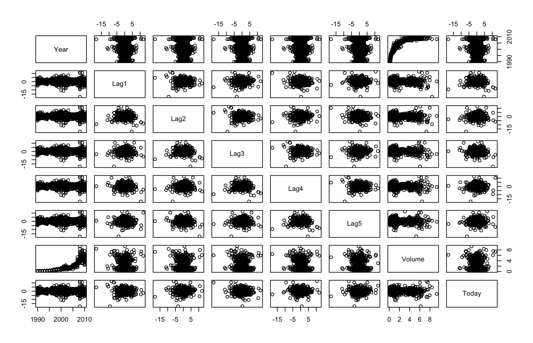
cor(Weekly[,1:8])Year Lag1 Lag2 Lag3 Lag4 Year 1.00000000 -0.032289274 -0.03339001 -0.03000649 -0.031127923 Lag1 -0.03228927 1.000000000 -0.07485305 0.05863568 -0.071273876 Lag2 -0.03339001 -0.074853051 1.00000000 -0.07572091 0.058381535 Lag3 -0.03000649 0.058635682 -0.07572091 1.00000000 -0.075395865 Lag4 -0.03112792 -0.071273876 0.05838153 -0.07539587 1.000000000 Lag5 -0.03051910 -0.008183096 -0.07249948 0.06065717 -0.075675027 Volume 0.84194162 -0.064951313 -0.08551314 -0.06928771 -0.061074617 Today -0.03245989 -0.075031842 0.05916672 -0.07124364 -0.007825873 Lag5 Volume Today Year -0.030519101 0.84194162 -0.032459894 Lag1 -0.008183096 -0.06495131 -0.075031842 Lag2 -0.072499482 -0.08551314 0.059166717 Lag3 0.060657175 -0.06928771 -0.071243639 Lag4 -0.075675027 -0.06107462 -0.007825873 Lag5 1.000000000 -0.05851741 0.011012698 Volume -0.058517414 1.00000000 -0.033077783 Today 0.011012698 -0.03307778 1.000000000Volumejest silnie dodatnio skorelowane zYear, reszta zmiennych jest bardzo słabo z sobą skorelowana, nie widać tutaj żadnych zależności.(b) Use the full data set to perform a logistic regression with
Directionas the response and the five lag variables plusVolumeas predictors. Use the summary function to print the results. Do any of the predictors appear to be statistically significant? If so, which ones?fit.log <- glm(Direction ~ . - Year - Today, data = Weekly, family = binomial) summary(fit.log)Call: glm(formula = Direction ~ . - Year - Today, family = binomial, data = Weekly) Coefficients: Estimate Std. Error z value Pr(>|z|) (Intercept) 0.26686 0.08593 3.106 0.0019 ** Lag1 -0.04127 0.02641 -1.563 0.1181 Lag2 0.05844 0.02686 2.175 0.0296 * Lag3 -0.01606 0.02666 -0.602 0.5469 Lag4 -0.02779 0.02646 -1.050 0.2937 Lag5 -0.01447 0.02638 -0.549 0.5833 Volume -0.02274 0.03690 -0.616 0.5377 --- Signif. codes: 0 ‘***’ 0.001 ‘**’ 0.01 ‘*’ 0.05 ‘.’ 0.1 ‘ ’ 1 (Dispersion parameter for binomial family taken to be 1) Null deviance: 1496.2 on 1088 degrees of freedom Residual deviance: 1486.4 on 1082 degrees of freedom AIC: 1500.4 Number of Fisher Scoring iterations: 4Tylko
Lag2jest istotne statystycznie o czym mówi p-value < 0.05.(c) Compute the confusion matrix and overall fraction of correct predictions. Explain what the confusion matrix is telling you about the types of mistakes made by logistic regression.
fit.log.probs <- predict(fit.log, type = "response")
attach(Weekly)
contrasts(Direction)
Up Down 0 Up 1fit.log.pred <- rep("Down", 1089) fit.log.pred[fit.log.probs > .5] = "Up" table(fit.log.pred, Direction)Direction fit.log.pred Down Up Down 54 48 Up 430 557 > (54 + 557) / 1089 [1] 0.5610652 > 557 / (430 + 557) [1] 0.5643364 > 54 / (54 + 48) [1] 0.5294118Elementy na przekątnej macierzy wskazują poprawne predykcje, elementy poza przekątną wskazują niepoprawne predykcje. W tym przypadku model ogólnie wykonał poprawnie 56.11% predykcji. Bardziej szczegółowo wykonał poprawnie 56.43% predykcji
Upi 52.94% predykcjiDown.(d) Now fit the logistic regression model using a training data period from 1990 to 2008, with
Lag2as the only predictor. Compute the confusion matrix and the overall fraction of correct predictions for the held out data (that is, the data from 2009 and 2010).train <- (Year < 2009) fit.log_2 <- glm(Direction ~ Lag2, data = Weekly[train,], family = binomial) fit.log_2.probs <- predict(fit.log_2, Weekly[!train,], type = "response") dim(Weekly[!train,])[1] 104 9fit.log_2.pred <- rep("Down", 104) fit.log_2.pred[fit.log_2.probs > .5] = "Up" t <- table(fit.log_2.pred, Weekly[!train, ]$Direction) tfit.log_2.pred Down Up Down 9 5 Up 34 56sum(diag(t)) / sum(t)[1] 0.625(e) Repeat (d) using LDA.
library(MASS)
fit.lda <- lda(Direction ~ Lag2, data = Weekly[train,])
fit.lda.pred <- predict(fit.lda, Weekly[!train,], type = "response")$class
t <- table(fit.lda.pred, Weekly[!train, ]$Direction)
t
fit.lda.pred Down Up Down 9 5 Up 34 56sum(diag(t)) / sum(t)[1] 0.625(f) Repeat (d) using QDA.
fit.qda <- qda(Direction ~ Lag2, data = Weekly[train,])
fit.qda.pred <- predict(fit.qda, Weekly[!train,], type = "response")$class
t <- table(fit.qda.pred, Weekly[!train, ]$Direction)
t
fit.qda.pred Down Up Down 0 0 Up 43 61sum(diag(t)) / sum(t)[1] 0.5865385(g) Repeat (d) using KNN with $K = 1$.
library(class)
fit <- knn(
    Weekly[train, "Lag2", drop = FALSE],
    Weekly[!train, "Lag2", drop = FALSE],
    Weekly$Direction[train]
    )
t <- table(fit, Weekly[!train, ]$Direction)
t
fit Down Up Down 21 30 Up 22 31sum(diag(t)) / sum(t)[1] 0.5(h) Repeat (d) using naive Bayes.
library(e1071)
fit.bayes <- naiveBayes(Direction ~ Lag2, data = Weekly[train, ])
pred <- predict(fit.bayes, Weekly[!train, ], type = "class")
t <- table(pred, Weekly[!train, ]$Direction)
t
pred Down Up Down 0 0 Up 43 61sum(diag(t)) / sum(t)[1] 0.5865385(i) Which of these methods appears to provide the best results on this data?
Najlepiej działają: regresja logistyczna i LDA. Obie metody klasyfikują najpoprawniej.
(j) Experiment with different combinations of predictors, including possible transformations and interactions, for each of the methods. Report the variables, method, and associated confusion matrix that appears to provide the best results on the held out data. Note that you should also experiment with values for $K$ in the KNN classifier.
# LDA fit.lda <- lda(Direction ~ Lag2 + Volume + Lag2:Volume, data = Weekly[train,]) fit.lda.pred <- predict(fit.lda, Weekly[!train,], type = "response")$class t <- table(fit.lda.pred, Weekly[!train, ]$Direction) sum(diag(t)) / sum(t)[1] 0.5384615# QDA fit.qda <- qda(Direction ~ Lag2 + Volume + Lag2:Volume, data = Weekly[train,]) fit.qda.pred <- predict(fit.qda, Weekly[!train,], type = "response")$class t <- table(fit.qda.pred, Weekly[!train, ]$Direction) sum(diag(t)) / sum(t)[1] 0.4711538# Naive Bayes - funkcja nie przyjmuje interakcji fit <- naiveBayes(Direction ~ Lag2 + Volume, data = Weekly[train, ]) pred <- predict(fit, Weekly[!train, ], type = "class") t <- table(pred, Weekly[!train, ]$Direction) sum(diag(t)) / sum(t)[1] 0.4519231# KNN set.seed(1) res <- sapply(1:50, function(k) { fit <- knn( Weekly[train, 2:4, drop = FALSE], Weekly[!train, 2:4, drop = FALSE], Weekly$Direction[train], k = k ) t <- table(fit, Weekly[!train, ]$Direction) sum(diag(t)) / sum(t) }) plot(1:50, res, type = "o", xlab = "k", ylab = "Fraction correct")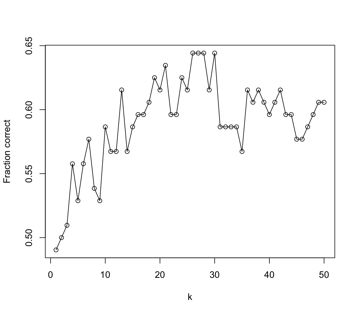
-
In this problem, you will develop a model to predict whether a given car gets high or low gas mileage based on the
Autodata set.(a) Create a binary variable,
mpg01, that contains a 1 ifmpgcontains a value above its median, and a 0 ifmpgcontains a value below its median. You can compute the median using themedian()function. Note you may find it helpful to use thedata.frame()function to create a single data set containing bothmpg01and the otherAutovariables.library(ISLR2) mpg01_ind <- data.frame("mpg01" = Auto$mpg > median(Auto$mpg)) Auto_2 <- cbind(Auto[, c(-1, -9)], data.frame("mpg01" = mpg01_ind))(b) Explore the data graphically in order to investigate the association between
mpg01and the other features. Which of the other features seem most likely to be useful in predictingmpg01? Scatterplots and boxplots may be useful tools to answer this question. Describe your findings.pairs(Auto_2) cor(Auto_2)cylinders displacement horsepower weight acceleration cylinders 1.0000000 0.9508233 0.8429834 0.8975273 -0.5046834 displacement 0.9508233 1.0000000 0.8972570 0.9329944 -0.5438005 horsepower 0.8429834 0.8972570 1.0000000 0.8645377 -0.6891955 weight 0.8975273 0.9329944 0.8645377 1.0000000 -0.4168392 acceleration -0.5046834 -0.5438005 -0.6891955 -0.4168392 1.0000000 year -0.3456474 -0.3698552 -0.4163615 -0.3091199 0.2903161 origin -0.5689316 -0.6145351 -0.4551715 -0.5850054 0.2127458 mpg01 -0.7591939 -0.7534766 -0.6670526 -0.7577566 0.3468215 year origin mpg01 cylinders -0.3456474 -0.5689316 -0.7591939 displacement -0.3698552 -0.6145351 -0.7534766 horsepower -0.4163615 -0.4551715 -0.6670526 weight -0.3091199 -0.5850054 -0.7577566 acceleration 0.2903161 0.2127458 0.3468215 year 1.0000000 0.1815277 0.4299042 origin 0.1815277 1.0000000 0.5136984 mpg01 0.4299042 0.5136984 1.0000000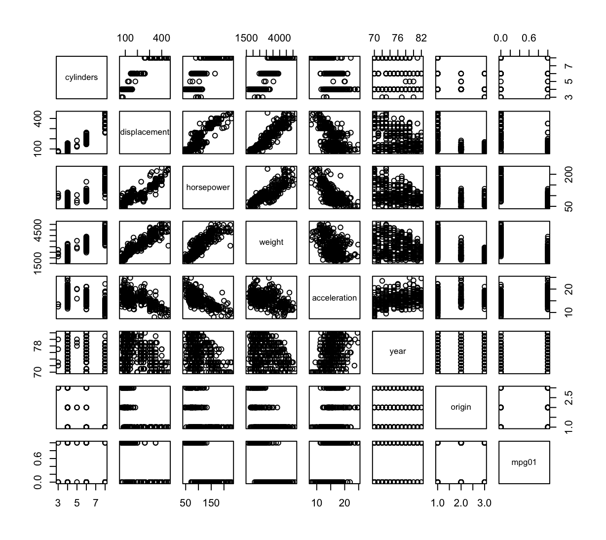
Istnieje silna korelacja między zmienną
mpg01i zmiennymi:cylinders,displacement,weight.(c) Split the data into a training set and a test set.
set.seed(1)
train <- sample(nrow(Auto_2), nrow(Auto_2) * 2 / 3)
(d) Perform LDA on the training data in order to predict
mpg01using the variables that seemed most associated withmpg01in (b). What is the test error of the model obtained?library(MASS) attach(Auto_2) fit.lda <- lda(mpg01 ~ cylinders + displacement + weight, data = Auto_2[train,]) fit.lda.pred <- predict(fit.lda, Auto_2[-train,], type = "response")$class t <- table(fit.lda.pred, Auto_2[-train, ]$mpg01) 1 - sum(diag(t)) / sum(t)[1] 0.1068702(e) Perform QDA on the training data in order to predict
mpg01using the variables that seemed most associated withmpg01in (b). What is the test error of the model obtained?fit.qda <- qda(mpg01 ~ cylinders + displacement + weight, data = Auto_2[train,]) fit.qda.pred <- predict(fit.qda, Auto_2[-train,], type = "response")$class t <- table(fit.qda.pred, Auto_2[-train, ]$mpg01) 1 - sum(diag(t)) / sum(t)[1] 0.09923664(f) Perform logistic regression on the training data in order to predict
mpg01using the variables that seemed most associated withmpg01in (b). What is the test error of the model obtained?fit.log <- glm(mpg01 ~ cylinders + displacement + weight, data = Auto_2[train, ], family = binomial) fit.log.pred <- predict(fit.log, Auto_2[-train, ], type = "response") > 0.5 t <- table(fit.log.pred, Auto_2[-train, ]$mpg01) 1 - sum(diag(t)) / sum(t)[1] 0.1145038(g) Perform naive Bayes on the training data in order to predict
mpg01using the variables that seemed most associated withmpg01in (b). What is the test error of the model obtained?library(e1071) fit.bayes <- naiveBayes(mpg01 ~ cylinders + displacement + weight, data = Auto_2[train, ]) fit.bayes.pred <- predict(fit.bayes, Auto_2[-train, ], type = "class") t <- table(fit.bayes.pred, Auto_2[-train, ]$mpg01) 1- sum(diag(t)) / sum(t)[1] 0.09923664(h) Perform KNN on the training data, with several values of $K$, in order to predict
mpg01. Use only the variables that seemed most associated withmpg01in (b). What test errors do you obtain? Which value of $K$ seems to perform the best on this data set?library(class) res <- sapply(1:50, function(k) { fit <- knn( Auto_2[train, 2:4, drop = FALSE], Auto_2[-train, 2:4, drop = FALSE], Auto_2$mpg01[train], k = k ) t <- table(fit, Auto_2[-train, ]$mpg01) 1 - sum(diag(t)) / sum(t) }) plot(1:50, res, type = "o", xlab = "k", ylab = "Fraction incorrect")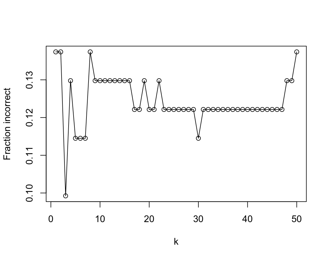
-
This problem involves writing functions.
(a) Write a function,
Power(), that prints out the result of raising 2 to the 3rd power. In other words, your function should compute $2^3$ and print out the results.Hint: Recall that
x^araisesxto the powera. Use theprint()function to output the result.Power <- function() print(2^3)(b) Create a new function,
Power2(), that allows you to pass any two numbers,xanda, and prints out the value ofx^a. You can do this by beginning your function with the line> Power2 <- function(x, a) {You should be able to call your function by entering, for instance,
> Power2(3, 8)on the command line. This should output the value of $3^8$, namely, 6,561.
Power2 <- function(x, a) { print(x^a) } Power2(3,8)[1] 6561(c) Using the
Power2()function that you just wrote, compute $10^3$, $8^{17}$, and $131^3$.> Power2(10,3) [1] 1000 > Power2(8,17) [1] 2.2518e+15 > Power2(131,3) [1] 2248091(d) Now create a new function,
Power3(), that actually returns the resultx^aas anRobject, rather than simply printing it to the screen. That is, if you store the valuex^ain an object calledresultwithin your function, then you can simplyreturn()this result, using the following line:return(result)The line above should be the last line in your function, before the
}symbol.Power3 <- function(x, a) { result <- x^a return(result) }(e) Now using the
Power3()function, create a plot of $f (x) = x^2$. The $x$-axis should display a range of integers from 1 to 10, and the $y$-axis should display $x^2$. Label the axes appropriately, and use an appropriate title for the figure. Consider displaying either the $x$-axis, the $y$-axis, or both on the log-scale. You can do this by usinglog = "x",log = "y", orlog = "xy"as arguments to theplot()function.plot(1:10, Power3(1:10, 2), xlab = "x", ylab = expression(paste("x"^"2")), log = "xy" )(f) Create a function,
PlotPower(), that allows you to create a plot ofxagainstx^afor a fixedaand for a range of values ofx. For instance, if you call> PlotPower(1:10 , 3)then a plot should be created with an $x$-axis taking on values $1$, $2$, . . . ,$10$, and a $y$-axis taking on values $1^3$, $2^3$, . . . ,$10^3$.
PlotPower <- function(x, a) { plot(x, Power3(x, a), xlab = "x", ylab = substitute("x"^a, list(a = a)), log = "xy" ) } -
Using the
Bostondata set, fit classification models in order to predict whether a given census tract has a crime rate above or below the median. Explore logistic regression, LDA, naive Bayes, and KNN models using various subsets of the predictors. Describe your findings.Hint: You will have to create the response variable yourself, using the variables that are contained in the
Bostondata set.library(ISLR2) library(MASS) library(e1071) library(class) attach(Boston) hcrim_ind <- data.frame("hcrim" = Boston$crim > median(Boston$crim)) Boston_2 <- cbind(Boston[, -1], data.frame("hcrim" = hcrim_ind)) set.seed(1) train <- sample(nrow(Boston_2), nrow(Boston_2) * 2 / 3) # Logistic Regression fit.log <- glm(hcrim ~ ., data = Boston_2[train, ], family = binomial) fit.log.pred <- predict(fit.log, Boston_2[-train, ], type = "response") > 0.5 t <- table(fit.log.pred, Boston_2[-train, ]$hcrim) sum(diag(t)) / sum(t)[1] 0.8934911summary(fit.log)Call: glm(formula = hcrim ~ ., family = binomial, data = Boston_2[train, ]) Coefficients: Estimate Std. Error z value Pr(>|z|) (Intercept) -41.102896 8.235788 -4.991 6.01e-07 *** zn -0.097831 0.046507 -2.104 0.035418 * indus -0.065145 0.059410 -1.097 0.272845 chas 0.255958 0.809541 0.316 0.751868 nox 55.531358 10.386451 5.347 8.97e-08 *** rm -0.729283 0.938617 -0.777 0.437173 age 0.022038 0.014381 1.532 0.125420 dis 1.116906 0.312413 3.575 0.000350 *** rad 0.680671 0.196508 3.464 0.000533 *** tax -0.005462 0.003226 -1.693 0.090489 . ptratio 0.335403 0.163873 2.047 0.040686 * black -0.010103 0.005428 -1.861 0.062684 . lstat 0.126713 0.060729 2.087 0.036930 * medv 0.237806 0.093429 2.545 0.010918 * --- Signif. codes: 0 ‘***’ 0.001 ‘**’ 0.01 ‘*’ 0.05 ‘.’ 0.1 ‘ ’ 1 (Dispersion parameter for binomial family taken to be 1) Null deviance: 467.04 on 336 degrees of freedom Residual deviance: 131.91 on 323 degrees of freedom AIC: 159.91 Number of Fisher Scoring iterations: 9Usunę zmienne dla których $p$-value jest za wysokie
fit.log <- glm(hcrim ~ zn + nox + dis + rad + tax + ptratio + black + lstat + medv, data = Boston_2[train, ], family = binomial) fit.log.pred <- predict(fit.log, Boston_2[-train, ], type = "response") > 0.5 t <- table(fit.log.pred, Boston_2[-train, ]$hcrim) sum(diag(t)) / sum(t)[1] 0.8698225summary(fit.log)Call: glm(formula = hcrim ~ zn + nox + dis + rad + tax + ptratio + black + lstat + medv, family = binomial, data = Boston_2[train, ]) Coefficients: Estimate Std. Error z value Pr(>|z|) (Intercept) -38.372956 7.524892 -5.099 3.41e-07 *** zn -0.099362 0.042410 -2.343 0.01914 * nox 49.956044 8.616373 5.798 6.72e-09 *** dis 0.924759 0.287264 3.219 0.00129 ** rad 0.738887 0.178274 4.145 3.40e-05 *** tax -0.006690 0.002895 -2.311 0.02085 * ptratio 0.277096 0.139538 1.986 0.04705 * black -0.009730 0.005274 -1.845 0.06504 . lstat 0.131937 0.055537 2.376 0.01752 * medv 0.164220 0.050523 3.250 0.00115 ** --- Signif. codes: 0 ‘***’ 0.001 ‘**’ 0.01 ‘*’ 0.05 ‘.’ 0.1 ‘ ’ 1 (Dispersion parameter for binomial family taken to be 1) Null deviance: 467.04 on 336 degrees of freedom Residual deviance: 136.04 on 327 degrees of freedom AIC: 156.04 Number of Fisher Scoring iterations: 9Jak na razie model zawierający wszystkie zmienne jest najlepszy, zostawię w modelu zmienne, które mają najwyższą korelację.
cor(Boston_2)zn indus chas nox rm age zn 1.00000000 -0.53382819 -0.042696719 -0.51660371 0.31199059 -0.56953734 indus -0.53382819 1.00000000 0.062938027 0.76365145 -0.39167585 0.64477851 chas -0.04269672 0.06293803 1.000000000 0.09120281 0.09125123 0.08651777 nox -0.51660371 0.76365145 0.091202807 1.00000000 -0.30218819 0.73147010 rm 0.31199059 -0.39167585 0.091251225 -0.30218819 1.00000000 -0.24026493 age -0.56953734 0.64477851 0.086517774 0.73147010 -0.24026493 1.00000000 dis 0.66440822 -0.70802699 -0.099175780 -0.76923011 0.20524621 -0.74788054 rad -0.31194783 0.59512927 -0.007368241 0.61144056 -0.20984667 0.45602245 tax -0.31456332 0.72076018 -0.035586518 0.66802320 -0.29204783 0.50645559 ptratio -0.39167855 0.38324756 -0.121515174 0.18893268 -0.35550149 0.26151501 black 0.17552032 -0.35697654 0.048788485 -0.38005064 0.12806864 -0.27353398 lstat -0.41299457 0.60379972 -0.053929298 0.59087892 -0.61380827 0.60233853 medv 0.36044534 -0.48372516 0.175260177 -0.42732077 0.69535995 -0.37695457 hcrim -0.43615103 0.60326017 0.070096774 0.72323480 -0.15637178 0.61393992 dis rad tax ptratio black lstat zn 0.66440822 -0.311947826 -0.31456332 -0.3916785 0.17552032 -0.4129946 indus -0.70802699 0.595129275 0.72076018 0.3832476 -0.35697654 0.6037997 chas -0.09917578 -0.007368241 -0.03558652 -0.1215152 0.04878848 -0.0539293 nox -0.76923011 0.611440563 0.66802320 0.1889327 -0.38005064 0.5908789 rm 0.20524621 -0.209846668 -0.29204783 -0.3555015 0.12806864 -0.6138083 age -0.74788054 0.456022452 0.50645559 0.2615150 -0.27353398 0.6023385 dis 1.00000000 -0.494587930 -0.53443158 -0.2324705 0.29151167 -0.4969958 rad -0.49458793 1.000000000 0.91022819 0.4647412 -0.44441282 0.4886763 tax -0.53443158 0.910228189 1.00000000 0.4608530 -0.44180801 0.5439934 ptratio -0.23247054 0.464741179 0.46085304 1.0000000 -0.17738330 0.3740443 black 0.29151167 -0.444412816 -0.44180801 -0.1773833 1.00000000 -0.3660869 lstat -0.49699583 0.488676335 0.54399341 0.3740443 -0.36608690 1.0000000 medv 0.24992873 -0.381626231 -0.46853593 -0.5077867 0.33346082 -0.7376627 hcrim -0.61634164 0.619786249 0.60874128 0.2535684 -0.35121093 0.4532627 medv hcrim zn 0.3604453 -0.43615103 indus -0.4837252 0.60326017 chas 0.1752602 0.07009677 nox -0.4273208 0.72323480 rm 0.6953599 -0.15637178 age -0.3769546 0.61393992 dis 0.2499287 -0.61634164 rad -0.3816262 0.61978625 tax -0.4685359 0.60874128 ptratio -0.5077867 0.25356836 black 0.3334608 -0.35121093 lstat -0.7376627 0.45326273 medv 1.0000000 -0.26301673 hcrim -0.2630167 1.00000000fit.log <- glm(hcrim ~ nox + rad, data = Boston_2[train, ], family = binomial) fit.log.pred <- predict(fit.log, Boston_2[-train, ], type = "response") > 0.5 t <- table(fit.log.pred, Boston_2[-train, ]$hcrim) sum(diag(t)) / sum(t)[1] 0.8579882Brak poprawy względem modelu zawierającego wszystkie zmienne.
# LDA fit.lda <- lda(hcrim ~ ., data = Boston_2[train,]) fit.lda.pred <- predict(fit.lda, Boston_2[-train,], type = "response")$class t <- table(fit.lda.pred, Boston_2[-train, ]$hcrim) sum(diag(t)) / sum(t)[1] 0.8402367# Naive Bayes fit.bayes <- naiveBayes(hcrim ~ ., data = Boston_2[train, ]) fit.bayes.pred <- predict(fit.bayes, Boston_2[-train, ], type = "class") t <- table(fit.bayes.pred, Boston_2[-train, ]$hcrim) sum(diag(t)) / sum(t)[1] 0.8047337# KNN set.seed(1) res <- sapply(1:50, function(k) { fit <- knn( Boston_2[train, c("nox", "rad"), drop = FALSE], Boston_2[-train, c("nox", "rad"), drop = FALSE], Boston_2$hcrim[train], k = k ) t <- table(fit, Boston_2[-train, ]$hcrim) sum(diag(t)) / sum(t) }) which.max(res) res[which.max(res)][1] 1 [1] 0.9704142Ostatecznie najlepiej klasyfikuje model KNN z $K=1$ ale ze zmniejszoną liczbą zmiennych:
nox,rad.